13.1 Overview
The presence or absence of a target variable distinguishes supervised from unsupervised machine learning. In supervised learning, each observation, each row of data, includes both feature values, X, and a known target value, y. The learning algorithm uses these labeled examples to learn a relationship between the features and the target. Then, from that learned relationship, make useful predictions of the target values for new observations. For example, a supervised learning model learns to predict a customer characteristic from information provided on an order form. The target variable defined by the customer characteristic supplies the outcome that the model is designed to predict.
What can we do when there is no target variable? Unsupervised learning explores patterns in the feature values without using a target to guide the analysis. There are still the X variables, the features, but no target variable, y.
Unsupervised learning: Methods for finding patterns, structure, or relationships in the feature data when no target variable is used to train the model.
Unsupervised learning can identify observations, such as for customers, with similar response profiles across the selected features.
13.1.1 Cluster Analysis
A common form of unsupervised learning is cluster analysis, which groups observations with similar measurements over multiple variables.
Cluster analysis: A set of methods that assigns observations to groups, called clusters, so that observations within a cluster are more similar to one another than to observations in other clusters.
In each cluster analysis, measurements on multiple variables form the basis of identifying the groups.
Features: Measured variables that describe each observation (people, products, countries, etc.).
Common applications of cluster analysis with the accompanying features include:
Retail-store planning: Group stores by sales volume, product-category sales, local demographics, seasonal demand, and customer traffic. The resulting store profiles can guide inventory allocation, staffing, merchandising, and distribution decisions.
Market segmentation: Group online customers by browsing activity, pages viewed, purchase frequency, average order value, and response to promotions. The resulting groups can identify, for example, frequent purchasers, occasional bargain shoppers, or customers at risk of becoming inactive.
Product assortment: Group products by sales volume, revenue, profit margin, purchase frequency, and patterns of co-purchase. The resulting groups can support assortment planning, product placement, and inventory management.
Health and patient profiles: Group patients by symptoms, laboratory measurements, diagnoses, treatment history, and health-care utilization. The resulting profiles can help researchers identify subgroups for further study or tailor care programs.
Geographic and community analysis: Group neighborhoods or regions by features such as population density, income, housing characteristics, age distribution, business activity, and transportation access. The resulting groups can inform public-policy planning, service delivery, or store-location decisions.
After identifying clusters, analysts can examine the feature profiles of the groups and decide whether they are interpretable and useful. How are the people (observations) similar? What are their common characteristics? In some settings, cluster assignments may later be used as labels for a supervised model that assigns new observations to similar groups.
13.1.2 Example
Consider a grocery-shopping example. Grocery chains can collect item-level transaction data when purchases are scanned at checkout. Suppose two shopper profiles have been identified for illustration: Healthy Food customers and Junk Food customers. The deliberately simple dataset records each customer’s spending for these two features: Fresh Vegetables and Chips, as shown in Table 13.1.
| CustomerID | Veggies | ChipsEtc |
|---|---|---|
| C0314 | 2.86 | 4.59 |
| C0971 | 2.50 | 7.01 |
| C1742 | 4.50 | 1.71 |
| C1917 | 7.74 | 2.81 |
| C2120 | 2.26 | 4.09 |
| C2738 | 8.89 | 2.34 |
| C2559 | 6.48 | 3.68 |
| C3686 | 1.62 | 4.47 |
The data for each customer are averaged across many shopping trips. A single shopping trip can be influenced by short-term needs, stock already available at home, or an unusual purchase. Averaging across trips can provide a more reliable description of each customer’s typical shopping pattern. A quick look at the data suggests a negative association between the two feature variables: customers who spend more on snack foods tend to spend less on fresh vegetables, and vice versa.
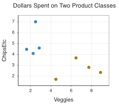
Because this example has only two features, we can visualize each customer in a two-dimensional scatterplot, with one axis for each feature. When plotted, each row of data becomes a point with its horizontal and vertical coordinates determined by that customer’s two feature values.
Feature space: A coordinate system in which each feature corresponds to a dimension (axis), and each observation corresponds to a point whose coordinates are its feature values.
The two-dimensional feature space in Figure 13.1 reveals an apparent separation between the two illustrated shopper profiles.
Next, fit a cluster analysis using only the two spending variables. For these idealized data, the evaluation measures support a two-cluster solution. The scatterplot in Figure 13.2 shows the observations, their assigned clusters, and the resulting center of each cluster computed by the cluster analysis. The points that comprise each cluster are separately colored.
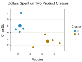
The center of each cluster summarizes the typical spending profile described by that cluster.
13.2 Distance Between Observations
How are clusters formed? There are many clustering methods based on some measure of similarity, of distance or dissimilarity across the selected features. Observations with smaller distances between their feature values are treated as more similar than observations with larger distances.
Similarity among the responses of two observations across the feature variables is assessed by the distance that separates them.
The smaller the distance between two sets of responses to the features, the greater their similarity, the basis for finding any distinct clusters of similar profiles of values for the observations across the features.
Several distance measures are available. Perhaps the most common distance measure used is Euclidean distance: the straight-line distance between two points in feature space.
13.2.1 Two Points
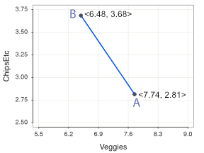
To illustrate Euclidean distance, consider two features so that the observations can be displayed in the feature space of a two-dimensional plot. Begin with two rows of data, each containing values for the features Veggies and ChipsEtc. When plotted, each row becomes a point: its horizontal and vertical coordinates are determined by that customer’s two feature values.
Consider two customer observations from Figure 13.2. To simplify our notation, refer to the two customers as A and B. The following small table shows their values for Veggies and ChipsEtc. We can use those values to calculate the geometric distance between the two points.
| CustomerID | Veggies | ChipsEtc |
|---|---|---|
| C1917 [A] | 7.74 | 2.81 |
| C2559 [B] | 6.48 | 3.68 |
How can we plot the two feature values for each customer?
Feature vector: An ordered set of feature values for one observation.
The Veggies and ChipsEtc values for each customer form a two-element feature vector. In a two-dimensional plot, these values also define the coordinates of the customer’s point: the first value gives the horizontal position and the second value gives the vertical position.
For Customer A and Customer B, the feature vectors:
\[A = <7.74, 2.81> \mathrm{and} \; B = <6.48, 3.68>\]
Plot the point for each customer and draw the line segment between them to create the two-dimensional visualization in Figure 13.3.
Now that we have the points, calculate the distance between them.
13.2.2 Euclidean Distance
Define the distance between Points A and B in a way that matches geometric intuition: the length of the straight line segment connecting them.
Euclidean distance: The straight-line distance between two points in a coordinate space.
The term refers to Euclidean geometry, associated with the ancient Greek mathematician Euclid and his work Elements, written around 300 BCE. Euclidean distance is a common choice for numerical data, including the K-means analysis presented in this chapter, though other distance measures can be more appropriate in other settings.
To calculate Euclidean distance in two dimensions, use the Pythagorean theorem. In Figure 13.4, the straight-line distance between Points A and B is shown as the blue line: the hypotenuse of a right triangle.
Pythagorean theorem: In a right triangle, the square of the hypotenuse length equals the sum of the squares of the other two side lengths.
The horizontal and vertical differences between the two points form the other two sides of the triangle. Square these differences, add the squared values, and take the square root to obtain the Euclidean distance. For Customers A and B, calculate the differences in Veggies and ChipsEtc; Figure 13.4 illustrates these two feature differences.
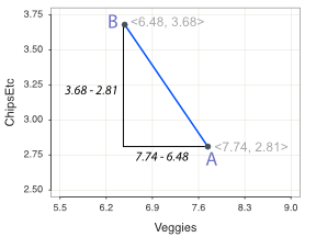
Apply the Pythagorean theorem to calculate the distance between Points A and B in Figure Figure 13.4) as the hypotenuse (long-side) of a right triangle.
\[\mathrm{distance}(A,B) = \sqrt{(7.74-6.48)^2 + (3.68-2.81)^2} = 5.47\]
To calculate Euclidean distance, first find the length of each side that meets at the right angle. Square those lengths, add the squared values, and take the square root of the sum.
13.2.3 Distance Generally Stated
The two-dimensional Euclidean-distance calculation generalizes to any number of features. If the analysis includes \(p\) features, each observation is represented by a point in a \(p\)-dimensional feature space.
First, consider two observations with two generic features, \(F_1\) and \(F_2\). Name the observations A and B, and label their corresponding feature values \(a_1\), \(a_2\), \(b_1\), and \(b_2\), as shown in the following table.
| Observation | F1 | F2 |
|---|---|---|
| Row_A | a1 | a2 |
| Row_B | b1 | b2 |
Use subscripts to identify the feature dimension. In this feature space, the first dimension corresponds to the first feature. Thus, \(a_1\) and \(b_1\) are the values for observations A and B, respectively, on the first feature—for example, Veggies.1
1 Coordinate geometry often labels the horizontal and vertical axes \(x\) and \(y\). In data analysis, subscripts commonly identify observations, features, or both, depending on the notation. Here, the letter identifies the observation and the subscript identifies the feature: \(a_1\) is the value of observation A on feature 1.
Represent the two feature values for the two observations as feature vectors:
\[A=<a_1, a_2> \mathrm{and} \; B=<b_1, b_2>\]
The feature space represents the numeric values from the data table as coordinates. It is often also called a vector space in this geometric context, although feature space is the more directly useful term here.
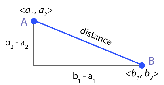
To calculate the Euclidean distance between two points, apply the Pythagorean theorem across the relevant feature dimensions. Begin with two features, as in Figure 13.5. The two legs of the corresponding right triangle have lengths \(|b_1-a_1|\) and \(|b_2-a_2|\). To calculate the Euclidean distance between observations A and B, calculate the difference on each feature, square each difference, sum the squared differences, and take the square root. The calculation begins with \((b_1-a_1)^2\) and continues through the \(p\)th feature, \((b_p-a_p)^2\).
\[\mathrm{Euclidean \; distance}(A,B) \; \mathrm{across \; two \; features} = \sqrt{(b_1 -a_1)^2 + (b_2 -a_2)^2}\]
In most applications, the analysis includes more than two features. Fortunately, dimensionality beyond two is not a problem as Euclidean distance straightforwardly generalizes from two dimensions to any number of features. For example, if Customer A has three features, then \(p=3\) and the customer is represented by the feature vector \(<a_1, a_2, a_3>\). Generalizing further, represent the data values of Row A for \(p\)-features in a \(p\)-dimensional space as vector \(<a_1, a_2, ..., a_p>\).
To calculate the Euclidean distance, apply the Pythagorean theorem feature-by-feature for the two observations (instances, objects, people). Begin with the squared difference of the first feature \((b_1-a_1)^2\). Then, for Rows A and B, continue summing through the sum of squared differences through the \(p^{th}\) feature, \((b_p-a_p)^2\), followed by the square root.
Euclidean distance as the application of the Pythagorean Theorem from Point A to Point B across \(p\) features: \[\sqrt{(b_1 -a_1)^2 + (b_2 -a_2)^2 \; + ... + \; (b_p -a_p)^2} \; = \; \sqrt{\sum\limits_{i=1}^p (b_i -a_i)^2}\]
This expression computes the Euclidean distance between any two feature vectors for any number of features. The underlying definition of distance remains the same. With more than two or three features, we cannot directly visualize the full feature space. We can, however, interpret clusters by examining their centroids across the features.
13.3 K-means Cluster Analysis
How can distances between observations provide the basis for cluster analysis? K-means is a straightforward distance-based clustering method. It represents each cluster by its center called a centroid.
Centroid: The center of a K-means cluster in which the coordinate for each feature is the mean of that feature among the observations assigned to the cluster.
The goal of K-means is to form \(k\) clusters such that observations within a cluster are close to their cluster centroid and more distant from other cluster centroids. The following section presents the perhaps surprisingly straightforward iterative algorithm from which the clusters are computed.
13.3.1 Solution Algorithm
A K-means cluster analysis requires the analyst to specify the number of clusters before fitting the model. The K-means algorithm then follows a simple iterative process:
- initialize cluster centers
- compute the distance of each point from each cluster centroid
- assign observations to their nearest center
- recompute the centers
- repeat until the solution no longer changes meaningfully.
Step 0: Initialize the cluster centroids. Begin by selecting one initial center for each of the \(k\) clusters. The process is random, though usually with the constraint that the initial clusters are at least somewhat separated from each other.

Step 1: Centroid distance. Calculate the Euclidean distance from each observation to each cluster centroid.
Step 2: Cluster assignment. Assign each observation to the cluster whose centroid is closest. Represent the centroid of Cluster \(j\) by the mean vector of features \(m_j\). Like an observation, the computed centroid is a point in the feature space.
Figure 13.7 shows the distances from one selected observation to both cluster centroids in the final solution. The observation is assigned to the cluster with the smaller distance.
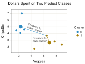
To get these sample-centroid distances, apply the computation of the distance formula of sample A with the computed centroid of the \(j^{th}\) cluster, computed across all \(p\) features.
\[\mathrm{Distance \; of \; Row \; A \; to \; Cluster \; j: \;}(A,m_j) = \sqrt{\sum\limits_{i=1}^p (a_i-m_j)^2}\]
Repeat the distance and assignment steps for every observation and every cluster. Each observation is assigned to the cluster with the smallest distance to its centroid.
Step 3: Centroid update. After all observations have been assigned, recompute every centroid. For each cluster, calculate the mean of each feature across the observations currently assigned to that cluster. The updated means become the new centroid coordinates.
Step 4: Repeat until convergence. Repeat the assignment and update steps until the algorithm converges or reaches the specified maximum number of iterations.
Converged solution: A K-means solution for which another assignment-and-update iteration produces no meaningful change in the centroids or cluster assignments.
Different initial centroids can lead K-means to different locally optimal solutions. So, for a fixed value of \(k\), evaluate several initializations and retain the solution with the lowest inertia. The model retains the solution with the smallest inertia.
13.3.2 Hyperparameter Tuning
Each K-means analysis begins with a specified number of clusters, \(k\). How can we select a useful value of \(k\) when its value must be specified before fitting the analysis? Treat the number of clusters as a hyperparameter: fit solutions across a reasonable range of values of \(k\), then compare them using fit measures, stability, and interpretability.
No single fit index identifies the universally “best” number of clusters. Instead, use multiple criteria to evaluate the proposed solutions. Because K-means is often computationally efficient, it is usually practical to evaluate several candidate values of \(k\) using multiple fit indices. Runtime still depends on the number of observations, features, candidate clusters, and initializations.
13.4 Evaluate Cluster Fit
How can we evaluate a clustering solution? A useful solution has observations that are close to their own cluster centroid and sufficiently separated from observations or centroids in other clusters. Consider two related concepts.
Cohesion: The compactness of a cluster—how close its observations are to one another or to their cluster centroid.
Separation: The degree to which one cluster is distinct from other clusters.
A useful clustering solution generally has high cohesion (small within-cluster distances) and high separation (large between-cluster distances).
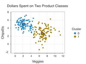
To illustrate, consider a larger, more realistic version of the Veggies and ChipsEtc data with nearly 200 observations. The visualization in Figure 13.8 contains nearly 200 points. Many observations form two visually distinct groups, but some lie near the boundary between the groups. These boundary observations may indicate overlap between the two groups, rather than clear evidence by themselves of a third cluster.
The two groups also differ in their variability. The observations that spend more on fresh vegetables appear more dispersed around their center than the observations concentrated on ChipsEtc. Some customers spend substantial amounts on both categories. This difference in spread is important when interpreting the clusters and evaluating their cohesion.
13.4.1 Inertia
In linear regression, a common measure of fit is the sum of squared errors (SSE): the sum of squared differences between observed target values and the values predicted by the model. K-means has no target variable, so it uses a different reference point. Each observation is compared with the centroid of the cluster to which it is assigned.
The relevant quantity is the distance from an observation to its assigned cluster centroid: the within-cluster distance.
Within-cluster residual: The difference between an observation and the centroid of its assigned cluster.
K-means evaluates a solution by summing the squared Euclidean distances from every observation to its assigned centroid.
Inertia: The total within-cluster sum of squared distances from observations to their assigned centroids.
During fitting, K-means alternates between assigning observations to their nearest centroid and recomputing the centroids. Each iteration reduces inertia or leaves it unchanged. When the algorithm converges, it has reached a locally optimal solution for the specified value of \(k\) and its particular initialization; a different initialization can produce a different local optimum.
To compare possible numbers of clusters, fit solutions across a range of values of \(k\) and record the inertia for each solution. The number of clusters is a hyperparameter because the analyst specifies it before fitting each model.
Inertia cannot, by itself, identify the preferred number of clusters. It always decreases or remains unchanged as \(k\) increases, because adding clusters gives the model more flexibility to reduce within-cluster distances. The useful question is whether an additional cluster provides enough reduction in inertia to justify the added complexity.
Elbow method: A visual heuristic that looks for a value of \(k\) after which additional clusters produce diminishing reductions in inertia.
Plot inertia against \(k\) to look for an “elbow”: a bend in the curve where the initial steep reduction in inertia begins to level off. The elbow is often subjective or unclear, so use it together with silhouette scores, cluster stability, and interpretability. Figure 13.9 illustrates an inertia plot created by evaluating multiple values of \(k\).
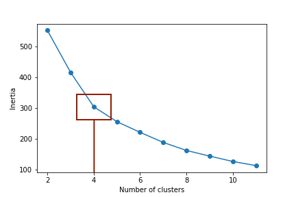
The inertia plot shows that the reduction in inertia becomes smaller after four clusters. This suggests that a four-cluster solution is worth considering in addition to the initially proposed two-cluster solution. The inertia plot alone does not decide between them.
13.4.2 Silhouette
Another fit index accounts for both cluster cohesion and separation.
Silhouette coefficient: A measure of how similar one observation is to its assigned cluster relative to the nearest competing cluster.
Compute a silhouette coefficient for each observation. The coefficient ranges from −1 to +1. Higher values indicate that the observation is, on average, closer to observations in its own cluster than to observations in the nearest other cluster. A value near 0 indicates that the observation lies near a boundary between clusters. A negative value indicates that the observation is, on average, closer to another cluster than to its assigned cluster.
For each observation, the silhouette coefficient compares two quantities:
\(a\): the mean within-cluster distance. For a selected observation, calculate its distance to every other observation assigned to the same cluster, then average those distances. A small value of \(a\) indicates that the observation is close to the other members of its assigned cluster.
\(b\): the mean nearest-cluster distance. For the selected observation, calculate its mean distance to the observations in each of the other clusters. Then select the smallest of these mean distances. The cluster that produces this smallest mean is the observation’s nearest competing, or neighboring, cluster. A large value of \(b\) indicates that the observation is well separated from its closest competing cluster.
The silhouette coefficient compares these two average distances. It does not use the distance to the centroids. Instead, the coefficient compares the observation’s distances to other observations.
The silhouette coefficient for an observation is
Silhouette coefficient: \(s = \dfrac{b - a}{max(a, b)}\)
When \(b>a\), the observation is closer to its own cluster than to the nearest competing cluster, so \(s\) is positive. As within-cluster distance \(a\) becomes small relative to between-cluster distance \(b\), \(s\) approaches 1. When \(a>b\), the coefficient is negative. Dividing by \(\max(a,b)\) normalizes the result so that silhouette values lie between −1 and +1.
To obtain an overall silhouette score for a clustering solution, average the silhouette coefficients across all observations. You can also average the coefficients within each cluster to evaluate which clusters are well defined and which contain boundary observations.
Unlike inertia, the average silhouette score does not necessarily rise or fall as the number of clusters increases. In Figure 13.10, the score decreases for some additional clusters and increases for others—for example, from 3 to 4 and from 7 to 8 clusters. Compare these scores with inertia, cluster stability, and interpretability when selecting a value of \(k\).
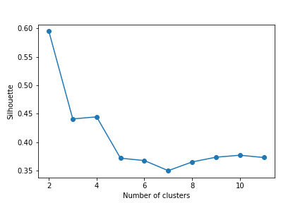
The average silhouette score drops substantially when moving from two to three clusters, then increases only slightly for four clusters. This pattern suggests that the two-cluster solution has the strongest separation and cohesion according to the silhouette criterion, while three- and four-cluster solutions may still be worth examining for interpretability.
Adding clusters does not produce a predictable pattern in silhouette scores. A higher score supports a more clearly separated solution, but it should be considered together with inertia, stability, cluster sizes, and practical usefulness.
For a selected solution, examine the individual silhouette coefficients across observations, for example with a histogram. Figure 13.11 displays the distribution of silhouette coefficients for the two-cluster solution. The plot can reveal whether most observations are well assigned or whether many lie near cluster boundaries.
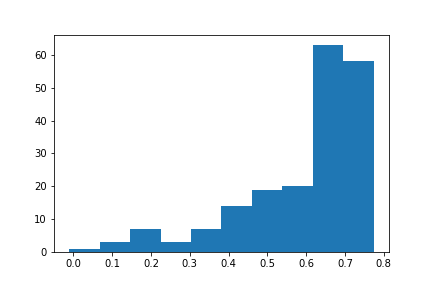
The good news for this interpretation is that most of the silhouette coefficients are above 0.4, and many above 0.6.
13.4.3 Selecting the Number of Clusters
Evaluate candidate clustering solutions using inertia and average silhouette score together.
Fit strategy: Prefer a solution that provides a meaningful reduction in inertia while maintaining a relatively high silhouette score, stable clusters, and practical interpretability.
Selecting the number of clusters requires judgment, but the decision should be informed by evidence. Examine inertia and average silhouette scores systematically across a reasonable range of values for \(k\). Also consider cluster sizes, stability across resampled data or initializations, and whether the cluster profiles answer a useful question.
Based on the hyperparameter-tuning results, consider the four-cluster solution shown in Figure 13.12.

The four-cluster solution provides a more detailed description of these customer purchase patterns. In the two-cluster solution, many observations vary continuously between the two broad groups. The four-cluster solution separates this variation into additional profiles.
For example, one cluster contains customers who purchase relatively many vegetables and few snack foods, while another shows the reverse pattern. A third cluster contains customers with moderate vegetable purchases and relatively high snack-food purchases. A fourth cluster contains customers who purchase substantial amounts of both categories. Verify the color and cluster-number labels in Figure 13.12 against the code: with four clusters, scikit-learn labels are typically 0, 1, 2, and 3.
Whether this additional detail is valuable depends on the intended use. For example, the cluster profiles could inform a targeted marketing campaign, merchandising decisions, or decisions about which product mix to emphasize at a new store location. The four-cluster solution is preferable only if these additional groups are sufficiently distinct, stable, and useful for the business question.
The larger number of clusters can make the original broad groups more specific, but the resulting profiles are descriptive patterns rather than fixed customer archetypes.
With a larger dataset, assess the stability and usefulness of the solution on new data. One approach is to fit K-means on a development sample, use predict() to assign new observations to the learned centroids, and then evaluate within-cluster distances and silhouette patterns in the new sample. With this small dataset, resampling or repeated analyses with different random samples can provide a more practical stability check than a single train/test split.