❝ Prediction is difficult, especially when dealing with the future ❞
1.1 The Machine

The ability to predict the unknown is a skill in demand. To make effective decisions today, managers need to know what will likely happen next week, next quarter, or next year. The better we predict, the better we plan, so the more successfully we provide for our customers and prevent problems from occurring. The predicted variable could be inventory level for a particular SKU, mortgage interest rate, shipment time, demand for a product, customer churn (loss), housing prices, clicking on a web page ad, employee turnover, population size, percentage of quality shipped parts, and many, many other possibilities.
The basis for prediction? One valid approach predicts from a time series, previous values of the variable that together are used to predict a future value of the same variable. Another approach, discussed here, is to learn how other variables with known values relate to the variable of interest with the unknown value. The intrigue is that a machine can now learn these relationships.
A machine? The word machine applied here is a trendy, almost cute, but effective reference to programmed instructions running on a computer. Note that these instructions as a concept do not even require a computer. Anything that the machine does a person can do as well. The only differentiating factors are that the person would take thousands of times longer to accomplish the same task, and can be more prone to error. The machine offers no underlying magic as every step of its doing machine learning is well understood. What it offers is error-free (if programmed correctly) and immensely faster processing.
This thorough understanding of machine learning algorithms does not extend to AI. We do not fully understand how AI works.
Machine: A computer that invokes a procedure according to pre-programmed instructions to accomplish a given task, such as learning.
People have always learned. Now machines can learn.
As applied here, learning proceeds from searching for patterns of related information from many existing examples of data. Except instead of you searching for these patterns from the data, the machine does the searching. And guess what? Given its staggeringly massive superiority in data processing speed, the machine uncovers many patterns much more effectively than can people. That is why we seek the machine’s help.
Machine learning (generically): Instruct the machine to identify patterns inherent in data, that is, the the relationships among variables.
What is the relation between ship time of an order to the carrier that does the shipping and the modality, ground vs. air? What is the relationship between salary and the time employed, the department of employment, and gender? Answering questions such as these is the motivation for doing machine learning.
1.2 Prediction Equation
1.2.1 Models
Pattern recognition applies to several types of machine learning analyses. One application predicts the unknown. Predict, for example, a person’s unknown height from their weight, albeit, imperfectly. These discovered relationship patterns enable a specific type of machine learning.
Supervised machine learning: Methods to develop the best possible prediction of an unknown value of the relevant variable from the related patterns with known values of other variables.
The machine expresses its learning as one or more equations that transform the related information into a prediction.
Model: One or more equations that computes an unknown value of a variable from the values of other variables.
The most straightforward prediction follows from a single equation.
The model transforms a set of entered numeric values into a predicted value, as illustrated in Figure 1.1.

To apply the model, enter the related information, then compute the predicted value.
1.2.2 Example
Consider an online clothing retailer who must correctly size the garment for a customer not present to verify fit. Returns annoy the customer and vaporize the profit margin for the retailer. Unfortunately, the customer sometimes omits from the online order form crucial measurements needed to fit a garment properly. If the customer omits their weight, the retailer wishes to predict this unknown value from the measurements the customer did provide.
Both a person’s height and chest size relate to their weight. Leveraging these relationships, the retailer’s analyst first specifies a general form of the model. One popular and simpler choice is a model defined as a weighted sum of the variables, here height and chest size, plus a constant, a linear model. What are the weights in the weighted sum that optimize the predictive accuracy of a customer’s weight? That discovery is the machine’s job.
For simplicity, this initial model derived from the data analysis in this example applies only to their male customers, the predominant customer type for this retailer. For additional simplicity, the form of the model is imposed to be linear according to the chosen estimation procedure. The result of the data analysis follows:
Predicted Weight = 3.80(Height) + 7.32(Chest) - 386.22
From examining the data values for each male customer’s recorded height, chest size, and weight, the machine learns the underlying relationship expressed as a weighted sum. From the linearity constraint, the machine learned (estimated) from the data the values of 3.80 and 7.32, plus the constant term of -386.22.
Supervised machine learning (specifically): The machine estimates (learns) the values of the weights in a prediction equation that best describe the relationship between the features, the predictor variables, and the target variable.
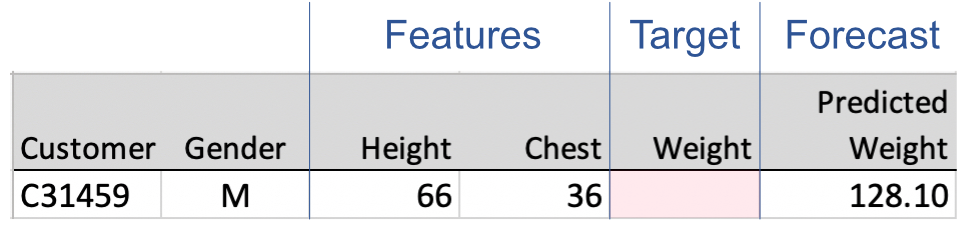
To apply the machine’s prediction model to a specific customer’s height and chest measurements, enter the corresponding data values, the measurements, into the prediction equation in place of the variable names. Suppose the customer reports a height of 66 inches and a chest measurement of 36 inches, illustrated in Figure 1.2.

From each specified entered value for every input variable in the model, the prediction model calculates a specific number, the prediction. The anticipated weight for a person 66 inches tall with a chest measurement of 36 inches is 128.10 pounds. We would not expect the person’s weight to be exactly 128.10 pounds, but we do expect it to be at least somewhat close.
1.3 Variables
The analysis begins with the choice of the variable for which to predict an unknown value.
People often say, “The variable that is predicted.”, but it is the values of the variable that are predicted.
Target: The variable’s values that are predicted.
Generically refer to the target variable as y, which assumes a specific variable name in a specific application, such as customer weight in the previous example. Traditionally, refer to the same y as the response variable, outcome variable, or dependent variable, among other names.
From what information does the prediction of the value of the target, y, proceed? In the online clothing retailer example, enter one customer’s height and chest size into the model.
Feature: One of typically several or even many variables from which to predict the value of the target variable.
Generically refer to the variables from which to compute the prediction as X, uppercase to denote that typically X consists of more than one feature: x1, x2, etc. Traditional references to the X variables include predictor variables, independent variables, explanatory variables or just predictor. The “cute” modern language replaces the meaningful word predictor with the more neutral word with less inherent meaning: feature.
The variables of interest for supervised machine learning models span a wide variety of applications. Table 1.1 lists some business scenarios, each with three features. Some of the target variables are continuous, measured on a quantitative scale. The values of other target variables in the table are labels, where each label defines a single category.
| y | x1 | x2 | x3 | |
|---|---|---|---|---|
| Continuous Target | ||||
| shipment | ship time | distance | carrier | modality |
| product | sales | discount % | radio ads | online ads |
| county | housing starts | interest rate | county population | average income |
| adult | weight | height | chest | neck |
| employee | salary | experience | department | gender |
| magazine | ad cost | audience size | percent male | median income |
| Categorical Target | ||||
| customer | stay/churn | tenure | total charge | payment method |
| part | accept/reject | length | finish | shift produced |
| web ad | click/ignore | gender | age | time on page |
| youtube video | watch/ignore | political affiliation | age | recently watched |
For a continuous target variable, predict a value that is as close to the actual value as possible. When that actual value becomes known, assess how close the predicted value is to the actual value. For labels, prediction is classification into the correct category. The many applications of machine learning for both continuous and categorical target variables contribute to its increasingly widespread use.
Beyond the form of the model, we need the data from which a chosen estimation procedure learns the model.
1.4 Data
The data for analysis encapsulate the experiences from which the machine learns. Gather data for all the variables in the model. To prepare for analysis, organize the data into a table, such as in Figure 1.3, perhaps using a standard worksheet app such as Microsoft Excel, or the free Apple Numbers for Apple devices, or the free and open-source LibreOffice Calc. For any of these three worksheet applications, save the file in the .xlsx format. List the data values for each variable in a single column. List the data values for each example in a single row.
Example: A partial data table that highlights a row of data values for the variables in the model, in this example, for a specific person.
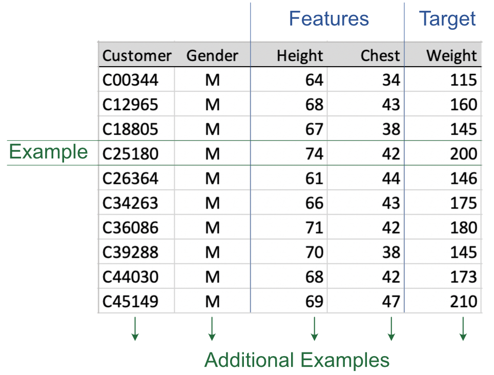
Be aware that the language that describes the data table is not consistent. Other names for a data example, a row of data in a data table, include sample, instance, observation, and case. Also, the ten rows of data shown in Figure 1.3, one row per customer, are a subset of a larger data set. In practice, the machine learns from many more examples, rows of data.
After reading the data into your preferred machine learning application, such as the open-source and free R or Python, estimate the model with a machine learning algorithm. From the data, the machine learning algorithm learns the relationship between the X variables and the known values of y. More specifically, the algorithm estimates the model weights from the sample data.
The purpose of this initial step is not to predict the values of the target variable y. The values of y are already present in the data table, so those values are known. There is nothing to predict for the observations used to estimate the model. Instead, prediction occurs later, when the estimated model is applied to new observations for which the values of X are known but the corresponding value of y is unknown.
Training data: Data from which the machine learns the relationships among all the variables in the model to construct a prediction equation.
The obtained prediction will not be perfect, but hopefully good enough to be useful. The goal is not to achieve perfect predictive accuracy, but instead better decision-making than not having the prediction.
1.5 Learn
The machine learns the patterns that relate the features to the target, expressed as a model. We inform the machine of only the general form of the model, such a weighted sum or linear model, before learning begins. From this general, imposed form, the machine analyzes the available training data to construct a specific model by estimating values of the weights. These weights optimize some aspect of predictive accuracy as it applies to the training data from which the model was derived.
We do not directly teach the machine.
The (estimation algorithm implemented on the) machine learns not by instruction but by example.
The machine learning software provides the instructions for the machine to learn by analyzing examples. For each row of the training data, the learning algorithm relates the values of the features to the corresponding value of the target variable. The target value for a row of data is the correct answer, the known value of y. This known value provides the “supervision” that guides the learning process. The algorithm then chooses weights for the features so that, averaged across all the training examples, the values of y computed from the model are as close as possible to the actual values of y.
Fitted value: Estimated value of y computed from the prediction equation, the model.
For each example, comparing this fitted value to the corresponding actual value becomes the basis for the machine learning the relationships.
Residual: Difference between the actual value of y, and the value of y fitted by the model.
The fitted value from the training data is not a prediction. The learning algorithm must already know the correct answer for each of many examples. On the contrary, prediction applies to unknown values.
The simplest machine learning procedure, linear regression, applies a fast, analytic procedure to directly estimate the weights of a proposed linear model, such as the weights 3.80, 7.32, and -386.22 in the clothing example. For more complex models and solution algorithms, the machine generally discovers relationships by trial and error, applying an iterative process called gradient descent. The algorithm repeatedly examines the training data to relate the X variables to y. Based on the form of the model specified by the analyst, the algorithm tries different values for the weights across a series of successive steps. At each step, it revises the weights to reduce the overall error averaged across all the training examples. Eventually, the machine concludes that it cannot find a new set of weights that meaningfully reduces the error beyond what has already been obtained.
There are many ways for the machine to learn from the data. The analyst can choose from many different:
- Types of models, such as linear regression, nonlinear regression, support vector machines, random forests, XGboost, and neural networks.
- Solution algorithms to estimate the weights of the selected model.
- Specific settings for the solution algorithm, each of which can be tuned to potentially improve predictive performance.
To learn machine learning is to learn how to invoke different types of models, estimation algorithms, and their associated settings to derive an effective predictive model from a given set of data. An expert in machine learning understands these models and corresponding algorithms, how they relate to each other, how to implement them for computer analysis, how to tune each procedure for better performance, and how to deploy the learned model to the relevant prediction setting. Attaining that level of expertise requires much practice and some mathematical training to better understand how the different procedures work.
Perhaps other algorithms, functional forms, or features would have led to a more useful predictive model in our online retail clothing example. Under the imposed functional form of a weighted sum, however, and given the chosen estimation algorithm, the resulting estimated weights – 3.80, 7.32, and -386.22 – minimize some function of the errors as applied to the training data.
That said, a basic introduction to machine learning and its Python implementation can provide the knowledge needed to begin doing actual, practical machine learning. For all of us, there is always more to learn, but there is also a core set of knowledge that allows us to begin as machine learning practitioners. Even if you do not develop the best, most optimized model, a valid model can still add value compared to having no model at all.
The word “valid,” however, carries much weight. It is always possible to develop an invalid model that performs poorly, fails on new data, or leads to worse decisions than having no model at all. For that reason, a basic introduction to machine learning must also include model evaluation strategies to help ensure that a developed model adds value rather than removes it.
1.6 Test
Teachers test students on their learning. The analyst tests the machine on its learning. People, and now machines, can try to learn, but was the learning successful? Maybe the person or machine could not apply a successful learning strategy, or maybe there was nothing there to learn, randomness rather than structure.
To validate an obtained model, test what the machine has learned on new examples, on previously unseen data. What is the source of this unseen data?
Testing data: A split of the original data held back from model estimation to test how well the machine can predict from new data.
Hopefully, in the era of big data, you have enough rows of data, examples, to split into two different sets, each large enough to fulfill their respective roles, training followed by testing.
The machine already knows the values of y for the training data, but not for the testing data. The analyst, however, knows the values of y for each set of feature values in both the training data and the testing data.
Prediction: The fitted value the model computes from the values of the features for data on which the model did not train.
In practice, the train/test data split is randomly generated, and then several other splits are also done, with the predictive power of the model evaluated on each split, and summarized by averaging the fit indices over all the splits.
Splitting the original data into training and testing data sets is one of the most fundamental concepts of data science. Because the machine does not use the values of y in the testing data to estimate the model, the analyst can evaluate the model’s true forecasting performance: how well the model works when y is treated as unknown. Of course, when the model is applied to generate real-world predictions, neither the machine nor the analyst knows the value of y, but the analyst now has a sense of the model’s likely forecasting error.
As with the training data, define an error as the difference between the actual value of y and the model’s fitted value, the comparison of what is with what the model specifies to be. In this situation, however, refer to the difference between what occurred and what was predicted to occur as forecasting error.
Figure 1.4 illustrates a prediction, with an unknown value of the target variable.
The need to evaluate the model with new data reveals an essential, but sobering, reality of machine learning. The average prediction error from new data is higher than the error from the model applied to the data from which the model was estimated. The reason for this worse performance is that the learning, or estimation, process is biased in favor of the data on which the model trained. Random variations across samples, known as sampling error, ensure that every sample is different. As a result, applying the model to new data introduces new random fluctuations not present in the training data.
Overfitting: The prediction model fits the training data too well, reflecting random perturbations of the training sample that do not generalize to new samples.
An overfit model can compute values of the target variable that closely match the known values in the training data, but then fail badly when predicting new data.
The goal of predictive, supervised machine learning is not to develop a model that minimizes errors on the training data, but instead to develop a model that minimizes errors on new data.
In pursuit of a continually better fit, the analyst may adjust and readjust the learning process and the model itself, running and revising the learning procedure over and over on the same training data. Evaluating predictive accuracy with testing data provides the necessary check on this process. The analyst may freely tune the learning process with repeated modifications on the training data, with one strong caveat: Always test the final model on new data. A model cannot be properly evaluated on data for which it has been trained.
1.7 Explain
The complexity of some machine learning algorithms renders their inner workings uninterpretable. A machine learning analysis can focus primarily on predictive accuracy, with less concern for understanding how the feature variables relate to the predicted value. With this emphasis, the specific process by which the feature values lead to effective prediction may not be of central interest.
Black box prediction: A prediction model that provides little or no information about how the values of the features relate to the target.
This lack of understanding may follow from a simple lack of interest, or from the overwhelming complexity of the prediction equations. Simpler models, such as models expressed as a weighted sum of the variables, tend to be more interpretable.
For some forms of machine learning, the process of transforming the values of the feature variables into a prediction is far too complex to represent as a single equation. For example, a neural network may require the estimation of not two weights, as in the previous example of the online clothing retailer, and not even a hundred weights, but tens of thousands, millions, or even billions of weights distributed across multiple equations layered together to form an interconnected network. In a large language model (LLM) such as ChatGPT, Claude, etc., this network generates text by repeatedly predicting the next word in its output, one word at a time. (More precisely, the LLM predicts aa word piece called a token.)
If the goal of the analysis is solely effective prediction, and if this effectiveness can be obtained without understanding the processes inside the black box, there may be no need for further explanation. Many scenarios, however, benefit from an explanation. Management and customers may want to know how the predictions are obtained. Regulators may demand such an explanation.
Explain: Understand how changes in the X variables relate to corresponding changes in the y variable.
The explanatory aspect of modeling attempts to answer why questions. Why did consumer demand drop for that product? Why did shipping costs rise? What attributes of a product enhance consumer satisfaction?
Prediction and explanation, moreover, are not mutually incompatible. Understanding the relationships among the variables beyond predictive accuracy is relevant in many, if not most, applications. Even when the emphasis is predictive accuracy, understanding each feature’s impact on the target can help the analyst choose features that more strongly influence the target variable, potentially leading to more accurate prediction.
For example, how much does weight increase, on average, for each additional inch of height and chest size? For each year that a person works at a company, how much, on average, does salary increase? How much do home sales decrease, on average, for each rise of one percentage point in the interest rate? More generally, which features have the most impact on the target variable?
Construct machine learning models to accomplish some combination of two goals:
1. Predict the value of a variable from other variables.
2. Understand/explain the relationship among variables.
When beginning a machine learning analysis, consider the purpose of the study. Is the emphasis on prediction or explanation and understanding of variable relationships? Often knowledge regarding both considerations are desired, but in some situations, construct the model to favor either prediction or explanation.
To maximize understanding of the relationships, enter a smaller number of more meaningful variables into the analysis. Much of modern machine learning focuses on predictive accuracy, with some models in some contexts built with hundreds of features. Still, the need for explanation and understanding remains in many contexts.
1.8 Procedure
Model construction for machine learning models follows a general procedure. Regardless of the specific model and the particular implementation of a learning algorithm, the overall predictive process remains the same.
- Prepare: Gather, clean, transform data as needed into a rectangular table, then split the data.
- Learn: Train the model on some of the data by minimizing a function of the discrepancy between the actual value of y with the value computed by the model.
- Validate: With the remaining data, calculate the predicted values, then assess the degree to which they match the true values.
- Deploy: If validated with sufficient accuracy, apply the model to real-world prediction.
Modern computing power and open-source software have made machine learning tools accessible to anyone with a personal computer or access to cloud computing. Not many years ago, applying machine learning often required the theoretical and mathematical expertise needed to develop and implement the algorithms directly, along with substantial computing resources. Today, many of those algorithms are efficiently packaged in user-accessible software modules that run with open-source languages such as Python and R.
Although some machine learning methods are computationally intensive, many useful analyses begin with relatively simple estimation algorithms that can work reasonably well needing just fractions of a second of computer time for smaller data sets. Machine learning software typically provides appropriate default settings for each algorithm, so the coding required to implement a basic analysis, while not trivial, is manageable. A model built by a beginner may not achieve the same predictive performance as a model built by an expert from the same data. Still, with modern free tools including AI, even a basic analysis can often produce a model that predicts more effectively than relying on judgment alone.
The technical accessibility of machine learning, however, does not by itself define the purpose of the analysis. Before beginning, we need data. However, more importantly, we need to know what the data are intended to help us understand or predict. The foundation of applying machine learning to a business problem is a precise statement of that problem and its scope. At the core of a successful machine learning analysis are the management insights gained from understanding how a specific predictive model can create value for the organization.