❝ Any data point you use to inspire a theory or question can’t be used to test that same theory. ❞
4.1 Fit that is Too Good
When the machine examines the data to learn the relationship between the features and the target variable, it constructs a model that achieves the optimal fit for prediction on the training data. However, the data values are for both predictive variables and the target variable. Because we already know the corresponding values of the target variable for the training data, there is no need to predict these already known values.
Instead, our primary interest is predicting from new data where the value of the target variable is unknown.
The data from which we estimate our model is not the data from which we wish to make predictions.
Optimal fit to the training data poses a central challenge in machine learning: the obtained fit to the data can be excessively good, minimizing too much error. Fit that is too good? Yes, when fit is assessed according to the data from which the machine learns, the resulting model might fit too well on the wrong data. Conversely, if the fit is too poor, the model may not be effective.
4.1.1 Sampling Error Example
Each data set samples from a larger population of data values. Two sources of influence contribute to each data value:
- Underlying population parameter such as the population mean or population slope coefficient: The signal, the stable characteristic that persists across samples.
- Sampling error: Noise that only exists in a single sample.
To illustrate, flip a coin 10 times and get six Heads. Flip the same coin again ten times and get four Heads. Is the probability of a Head 0.6 or 0.4? Trick question. The answer is neither.
The actual population value, the true probability in this example, shapes the outcome, but so does the noisy sampling error. A data sample reflects both the reality of the underlying population characteristics as well as the random fluctuations of sampling error. Different samples yield different results.
Presume the coin is fair. Flipping a fair coin 10 times results in 5 Heads only for 24.6% of the multiple sets of 10 flips. The random fluctuations imposed by sampling error imply that the population value of 5 Heads out of 10 flips is more often not obtained than it is obtained. Even for only 10 flips, the sample proportion does not equal the population probability more often than not. With a very large number of flips, the sample proportion of Heads rarely equals the true probability of a Head. The noise of sampling error obscures reality.
4.1.2 Training Data
A supervised machine learning algorithm searches for patterns more sophisticated than a simple coin flip probability. From a sample of data, the algorithm estimates the equation that predicts the value of the target variable from the values of the predictor variables.
A successful model fits the data, accounting for the target variable values on which it trained. Least-squares estimation provides the mathematically guaranteed optimal fit of the estimated model to the data on which it learned the model. This procedure chooses values of the \(y\)-intercept and slope coefficients that minimize the sum of the squared residuals, \(\Sigma e_i^2\).
However, there is a catch. Unfortunately, this minimization of error takes advantage of chance to produce an optimized outcome only for that particular sample. The artifacts present in a specific sample can severely hinder the model’s ability to make accurate predictions in real-world scenarios on new data. Any set of estimates for the \(y\)-intercept and slope coefficients that necessarily emerges from data with random sampling error is specific to a particular sample dataset, the training data.
4.1.3 Generalize
We care about much more than our ability to describe patterns in the training data. Machine learning is successful only to the extent that it uncovers patterns that generalize to new data. Otherwise, we engage in a form of sophistry. If our model does not generalize beyond the training data, our silly accomplishment is the ability to estimate the value of \(y\) from data in which we already know its value!
This new, previously unseen data presents new random sampling fluctuations unrelated to those randomly distorting the training data. We only care about the population truth that is partially obscured by one arbitrary sample.
If sampling error strongly influences the estimated model, then the estimated parameter values of the same model, when estimated on new data, would change much from sample to sample. A model that depends much on the random characteristics of a specific sample adds much uncertainty to any single prediction.
The estimated model, so elegantly optimized to maximize fit to the training data sample, is not optimized for any new sample for which to predict.
Optimization is great, but limited to the one sample of data.
We do require satisfactory fit of the model to the training data. A model that cannot recover the values of \(y\) on its training data cannot recover the values of \(y\) in the more challenging scenario of new data that it has not before encountered. We require more, however, than satisfactory performance on the training data. A model that adequately fits the training data may or may not generalize to new data sampled from the same population.
The evaluation of a model requires new data, entirely separate from the training data.
Applying the model optimized on the training data to new data, and new sampling error, generally weakens fit and performance. Yet a successful model must generalize its predictive efficiency beyond the training data to predict outcomes from new data, previously unseen data where the target values are not available to the model.
Avoid the artifacts!
A successful machine learning analysis identifies patterns in the data that generalize to new data sets and avoids patterns that only exist in the sample data from which the model was trained.
Achieving the optimal balance between fitting artifacts and generalizing the model to a new sample for true prediction is a central challenge of the machine learning analyst.
4.1.4 Over- vs Under-Fit
More complex models can increase fit. One possibility increases the complexity of a model by increasing the number of predictor variables. Another possibility adds curvilinearity to what was previously a linear model, such as by squaring the values of a predictor variable. The good news and simultaneously the bad news is that the more complicated the model, the more opportunities for the estimating method to alter the model’s weights to improve the fit. Better fit is good but usually not the best possible fit.
Especially for small data sets, model complexity can increase to the extent that all the fitted values perfectly match the training data.
An essential principle of machine learning for model fit is that we do not seek the very best fit of the model to the training data. An overfit model captures too much random noise in the data, the sampling error. Any elation after obtaining a great fit of an overfit model to the training data quickly fades when evaluating predictions applied to new data. Too good a fit to training data transforms into a poor fit when predicting with new data.1
1 Section 11.3 provides an example of overfitting in another context, a decision tree model.
The variance of the model reflects its sensitivity to the training data. The estimated high variance model changes much from sample to sample, rendering the model ineffective for predicting new data. A model with low variance generalizes appropriately to new data and so becomes a candidate for predicting unknown values.
Obtaining the best fit possible without overfitting is a central consideration for building robust and accurate supervised machine learning models.
The optimal predictive model estimated from the given training data minimizes error on new data, not training data.
The opposite problem of overfitting is a model that is too simple for the data.
The underfit model fails to detect useful information in the data.
A too-simplified or inappropriate model is biased, it does not detect the complete pattern of the relationship between the features and the target. The underfit model underperforms both the training data and when applied to new data such as test data.
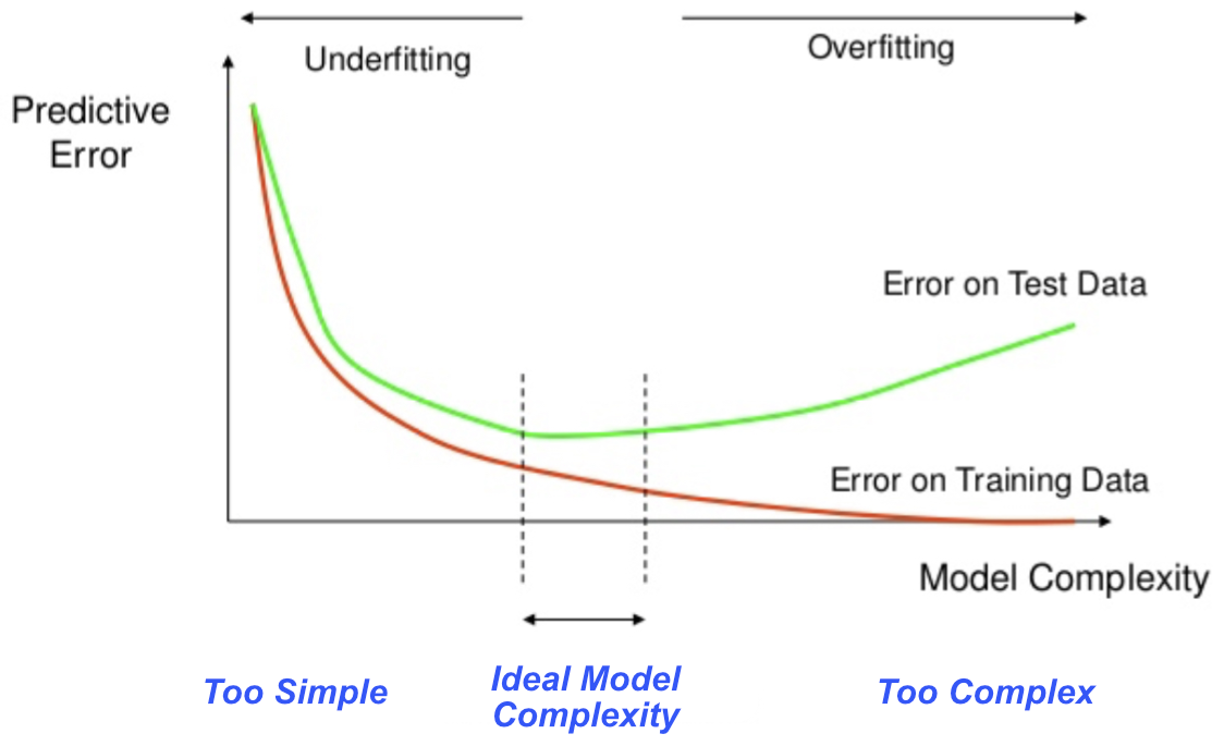
Figure 4.1 illustrates the dialectical tension between competing motivations of simultaneously attempting to minimize underfitting and overfitting.

The ideal model is one with low variance and low bias. A model with low bias accurately captures the underlying patterns in the training data, while a model with low variance generalizes well to new data. Our goal is to fit the given data and ensure that our results generalize to new data for accurate prediction.
Achieving the optimal balance between bias and variance is crucial for building effective machine learning models. However, finding this ideal is challenging because minimizing one criterion often inflates the other. For instance, if the additional revisions only respond to chance data fluctuations, the model’s fit to the training data increases as its generalizability to predicting new data decreases. A successful machine learning model strikes a balance between overfitting and underfitting to achieve satisfactory prediction accuracy. Too much model complexity absorbs quirky aspects of the training data. Too little model complexity fails to account for the relations among the variables as they exist.
This tension between these two competing tendencies of fit results in a fundamental principle of machine learning.
The chosen model is usually not the best-fitting model to the data. Instead, the model should be as simple as possible without meaningfully compromising fit, but not simpler. To the extent possible, select a model that maintains both low bias and low variance. The analyst must successfully manage this balance given the available data to create a model that can be successfully applied to real-world prediction.
Overly complicated models tailored to the minute specifics of a data set are susceptible to high variance. An overfit model has small residuals with the training data but much error when predicting the target variable in new data. Conversely, an underfit model is too simple, with too much bias.
This tension between over- and under-fitting eases as the advantage of large samples increases. With more data, the analyst can create a more complex model without taking advantage of chance or overfitting.
Flip a fair coin 1000 times instead of 10 times. Getting 600 heads 1000 flips is way less unlikely that realizing 6 heads out of 10 flips.
The need for predictability leads to a different evaluation than the mean-squared error of the model to the training data, the topic pursued next.
4.2 Data Splitting
4.2.1 Hold-Out Sample
Play with your data. Develop insights. Be inspired. Build a model. Revise the model to fit better. Revise the model again. Try a different machine learning algorithm. You now have your model that explains interesting stuff, at least in the data from which the model was developed. However, how can you know if your model is overfitted? Did you discover something real, or were you only playing with data and nothing more?
There is a simple but quite effective technique to evaluate overfitting. The technique involves no equations that apply sophisticated mathematical theory. Instead, simply check your understanding with new data to verify that you successfully revealed structure that generalizes to new data for successful prediction.
Where do we find these new data values to evaluate predictive performance? One of the essential practices of machine learning splits the original data. The modern era of data analytics often provides enough data to split the data and retain a reasonable number of samples in each split.
Begin each machine learning analysis with at least one random partition of the original, full data set.
From the training data the machine (estimation algorithm implemented on the computer) learns (estimates) your model. The hold-out sample is for testing the model.
The analyst knows the target values of the testing data, but the machine does not, which provides the basis for evaluating true prediction accuracy. If true prediction performance applied to the testing data decreases much relative to training data performance, the estimated model has modeled statistical noise. The model has overfitted the data.
To evaluate a model, examine the fit indices on the testing data and also compare the testing data fit to the training data fit. The test data hopefully confirms what you discovered in the training data. If your discoveries generalize, then success! If not, back to the training data to hopefully develop better insights.
Usually retain about 70% of a random split of the data for estimation, and then the remaining 30% of the data for validation. Too small of a training data sample yields poor estimates. To evaluate your model estimated on the training data, apply the model to the validation (testing) sample. Then evaluate fit with a standard fit index such as \(SSE = \Sigma e^2\) and/or \(MSE\) or \(s_e\).
How to select features? Always better to drop features that do not contribute to model fit after the model is estimated. The only way to be entirely sure that a feature should not be in the model is to see how it performs in the model estimation.
Avoid data analysis until the data are split into training and testing data sets. The goal is to develop the model only from training data. We can revise and modify our model indefinitely, as long as we test on data from which no modifications have been made – the true prediction situation.
When testing the model on data previously unseen by the model, all aspects of that data must have been unseen, just as in a real-world prediction scenario. Otherwise the data is said to leak from training to testing data. Making decisions regarding the model based on all the data then by definition includes both training and testing data. Best to make decisions regarding model estimation only from the training data. Otherwise the model is estimated from information that would, in a completely new prediction situation, be unavailable.
In practice, however, if you have a huge data set and a model with many predictors, and if applying more computationally intensive models than linear regression such as neural networks, there may be a need to reduce computation time. In that situation, without doing any model estimation, perhaps eliminate some features that violate the two properties of relevance and uniqueness before model specification and estimation.
4.2.2 k-fold Cross-Validation
4.2.2.1 Concept
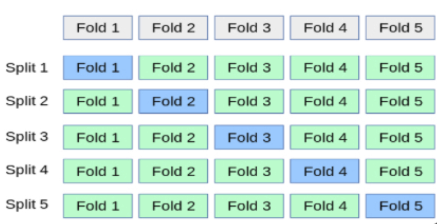
The \(k\)-fold cross-validation process extends the concept of cross-validation on a single hold-out sample to \(k\) separate training and hold-out samples. Multiple hold-out samples mitigate the impact of randomness of any one sample.
For a moderate-size sample, a typical value of \(k\) is 5, or, for smaller samples, 3. For \(k=5\), randomly partition the data into five different sets of about equal size. Each set is called a fold. Train the first model on the remaining folds, two through five, then use the first fold as the hold-out testing set. Evaluate this trained model by predicting the values of \(y\) on the first fold.
Then, define the second fold as the hold-out sample, and use the first fold, and folds three through five as the training data. Evaluate the model by applying the estimated model to the second fold. Repeat this process for all five folds.
Figure 4.2, from the official Python sklearn documentation, illustrates the \(k\)-fold procedure.
For a fit statistic, the best single statistic of model fit is the average of a chosen fit statistic from applying the model to the test data sets over the \(k\) different analyses.
4.2.2.2 Example
Figure 4.3 shows the corresponding cross-validation output.
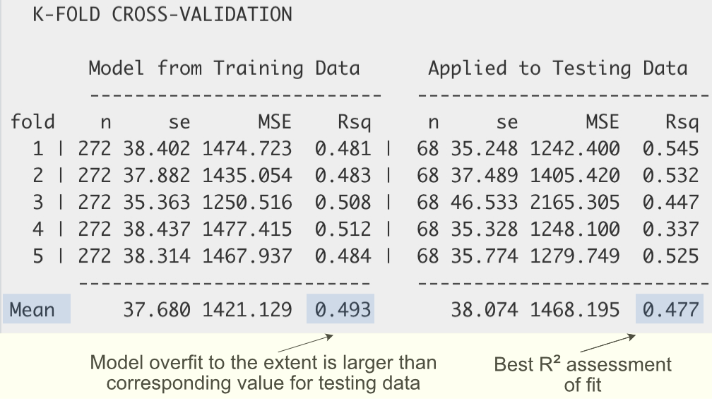
The best assessment of model fit in terms of \(R^2\) is its average value over all five analyses, the value of 0.477 in this example. There is also considerable variability of the five \(R^2\) values from the individual analyses, ranging from \(R^2=0.337\) to \(R^2=0.545\). The explanation for this variability is the presence of an outlier in these data values. For the low value of \(0.337\), the fourth analysis, the outlier was likely present in the testing data fold.
Evaluate the extent of overfit by comparing the value of \(R^2\) averaged over the training data analyses, \(0.493\), to that of the testing data, \(0.477\). As expected, the training data fit is higher than for the testing data but not substantially higher. There is some overfit, but not much.
Of course, the same logic for the evaluation of fit applies to the other two reported fit indices in Figure 4.3 as well. For the standard deviation of the residuals, \(s_e\), and for the Mean Squared Error, MSE, smaller values indicate better fit. In this example, the training data value of \(37.680\) is smaller than the value of \(38.074\) for the testing data, but not so much smaller. Similarly, for the Mean Square Error, MSE, the average training data value of \(1421.129\) is smaller than the corresponding testing data value of \(1468.195\), but not so much smaller. There is some overfit as expected, but not too much.
In subsequent material on a topic called hyperparameters we generalize to situations where three basic data splits are needed: training data, validation data, and testing data. And, within those three basic splits, we are also free to pursue \(k\)-fold cross-validation.
4.3 Prediction Intervals
Statistical estimates are just that – estimates.
Always report each statistical estimate within a band of uncertainty.
Report the confidence interval for a statistic such as a slope coefficient, previously discussed, and the error band for the data range about the predicted value.
The construction of these intervals depends on their underlying sources of error, which depends on the distinction between training data and new data from which the model has not been trained, the testing data.
4.3.1 Confidence Interval of a Conditional Mean
The fitted value \(\hat y\) is a mean, of which we can apply to different sets of data.
A conditional mean of \(y\) is the mean for just those rows of data where \(x\) equals a specific value such as 4 or -15.8 or whatever, generically referred to as \(x_p\). For example, a conditional mean of weight is the mean weight of all people who are 70.5 inches tall. Another conditional mean is the mean weight of all people who are 64 inches tall.
Why do we care about the conditional mean?
Each point on a regression line is a conditional mean assuming linearity.
Particularly for a small data set, there may only be one value of \(y\) for a given value of \(x\). In our simple 10 sample data set of height and weight, only one person had a height of 70.5 inches, so there is only one corresponding value of \(y_{70.5}\). Yet there is a hypothetical distribution of many, many values of \(y\) at \(x=70.5\), an entire distribution of \(y_{70.5}\)’s, that is, the weights of people who are 70.5 inches tall. The value of \(\hat y\) for \(x=70.5\) is the mean of that distribution (assuming a linear relationship).
The regression line is a sample result determined by the sample values of \(b_0\) and \(b_1\). Each sample obtain a different estimated model. For a given value of \(x\), \(x_p\), different estimated values of \(b_0\) and \(b_1\) result in a different fitted value, \(\hat y\), for \(x_p\). That is, \(\hat y\) varies from sample to sample, the result of sampling error. Denote the standard deviation of this distribution of \(\hat y\)’s just for values \(x_p\), as \(s_{\hat y_p}\). Sampling error applies to the construction of the corresponding confidence interval of the conditional mean.
Each value of \(x\) yields not only a different value of \(\hat y\), but also, in general, a different sized confidence interval about that \(\hat y\). As Figure 4.4 illustrates, for the value close to the mean of \(x\), there is a relatively small amount of fluctuation from sample to sample of the point on the regression line, the fitted value.
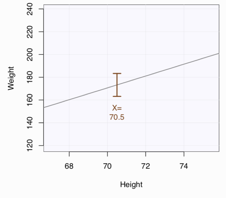
The further the value of \(x\) lies from its mean, the larger the fluctuations of the fitted value across the hypothetical samples. As Figure 4.5 illustrates, the confidence interval of the conditional mean, the point on the regression line for the corresponding value of \(x\), becomes larger as the value of \(x\) becomes farther from its mean.
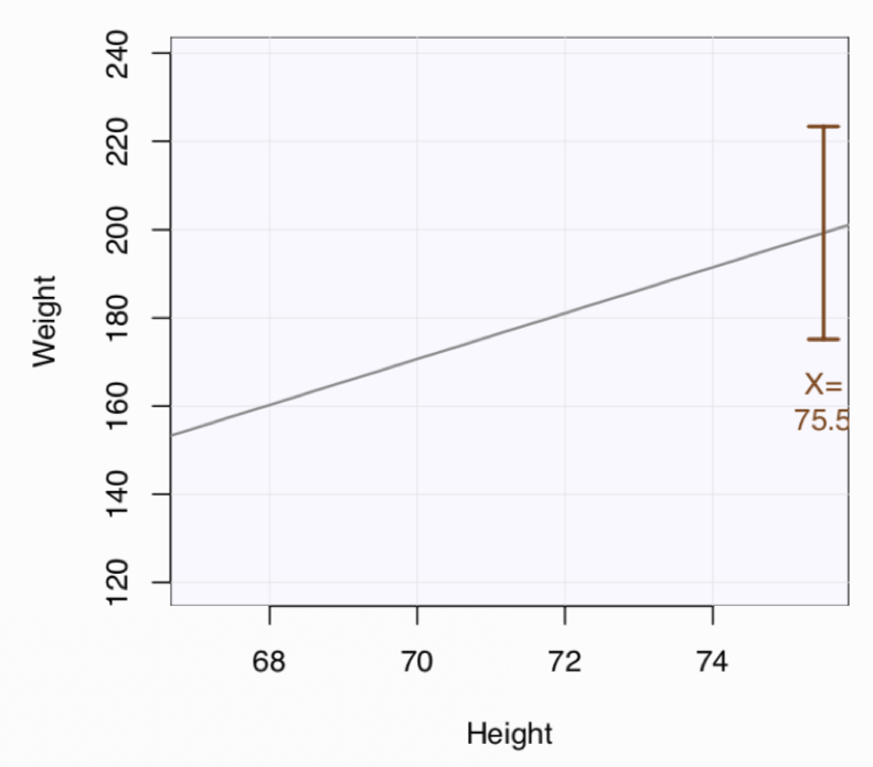
Figure 4.6 illustrates, the fluctuation of the sample regression line from sample to sample tends to resemble a teeter-totter.
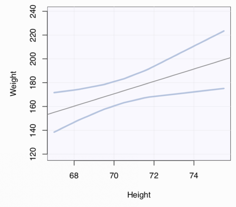
The fluctuations of the regression line across samples, that is differences in estimates \(b_0\) and \(b_1\), result in the variability of the physical positioning of the regression line. Of even greater interest is the intervals that contain the predicted value.
4.3.2 Fitted vs. Predicted Values
Compare the following two ways to apply the regression model, somewhat confusing because the same notation applies to the same computation, but different concepts. Fitted values are computed from the same model regardless if using \(x\) values from the training data or from new data, such a testing data, true prediction. The distinction is important because the fitted values from testing data are generally not as close to the corresponding true data values as are the fitted values computed from training \(x\) data values.
Distinguish between the two corresponding types of residuals, again both computed identically.
The interpretation of these values from training versus new data differs because the sources of error that underlies these values differ. Unfortunately, tradition relies upon the same notation for two separate concepts, a confounding that can lead to confusion.2 Yes, compute with the same procedure the fitted and predicted values: input a value of \(x\) into the equation of the model to derive the corresponding value of \(\hat y\). Similarly, compute the training residuals and prediction residuals the same, \(y_i = \hat y_i\). But the meaning of applying the procedures of computing \(\hat y_i\) and associated \(e_i\) from the training data \(x\) is different from the meaning of applying that same procedure to \(x\) from new data, such as the testing data.
2 To clearly explicate these two distinct concepts, fitted and predicted values, requires two different notations. One possibility is \(\tilde y_i\) for the fitted value of \(y_i\) and \(\hat y_i\) for the predicted value of \(y_i\). But then it is not up to me to re-define standard notation, so I will continue to use \(\hat y_i\) for both applications.
Training error, assessed globally with \(\Sigma e^2\), or some derivative thereof, such as \(s_e\), describes the size of the residuals for the training data. Training error applies to a single sample, that is, without consideration of any sampling error that underlies that sample. Sampling error is different. It describes the variability of a point on a regression line for a given value of \(x\) across repeated samples.
4.3.3 Standard Error of Prediction
The prediction of a given, specific value of \(x\), \(x_p\), is \(\hat y_p\), the same prediction as the conditional mean, the point on the regression line. The value of \(y_p\), however, does not lie on the regression line, but is part of the scatter in a scatterplot. The prediction for both a conditional mean on the regression line and a specific data value \(y_p\), generally off of the line, is \(\hat y_p\). However, the corresponding underlying sources of errors differ.
The prediction of a conditional mean on the regression line only is influenced by a single source of error, the sampling error inherent in the instability of the sample estimates for the intercept and slope, \(b_0\) and \(b_1\). However, the size of the typical residual, when applied to a prediction of an individual data value in a new sample from a line estimated from another, older sample, results from two sources of error.
The size of a prediction interval for a fitted value depends on two sources of random variability.
- The extent of sampling error of the conditional mean, the point on the regression line that corresponds to the value of \(x\) of interest
- The extent of training error, assessed by \(s_e\)
Training error is assessed free of sampling error, calculated from just a single sample of training data. To assess the accuracy of prediction, however, requires both sources of error.
The variability of the predicted value over multiple samples reflects both the inherent training error and the sampling error resulting from the instability of the sample estimates of \(b_0\) and \(b_1\) over repeated samples.
The interval about a predicted individual value of \(y\), \(\hat y_i\), depends on the joint assessment of both training error and of sampling error. The precise contribution of training error and sampling error to the standard error of prediction, \(s_{\hat y_{p,i}}\) follows.
Training error itself is assessed by the standard deviation of the residuals, \(s_e\), and sampling error is assessed with the standard error of the conditional mean, \(s_{\hat y_p}\). The two types of error are independent of each other, combining additively in the equation of the standard error of prediction.
The corresponding standard deviation of the residuals is generally larger for testing data than training data.
The statistic of ultimate interest for assessing prediction accuracy is the standard error of prediction, which incorporates the two distinct sources of error. Unfortunately, the standard error of prediction is larger than both the standard deviation of the residuals, \(s_e\), and the standard error of the corresponding conditional mean, \(s_{\hat y_p}\). Worse, increasing sample size reduces the standard error of the conditional mean, but not of training error.
This combination of two sources of errors expresses the extent of error likely encountered in an actual prediction situation. Compute confidence/prediction intervals from the same basic form, where the margin of error, \(E\), is about two (precisely \(t_{.025}\), \(df=n-2\) for a one predictor model) standard errors on either side of the estimate.
\[E = (t_{.025})(\textrm{standard error})\]
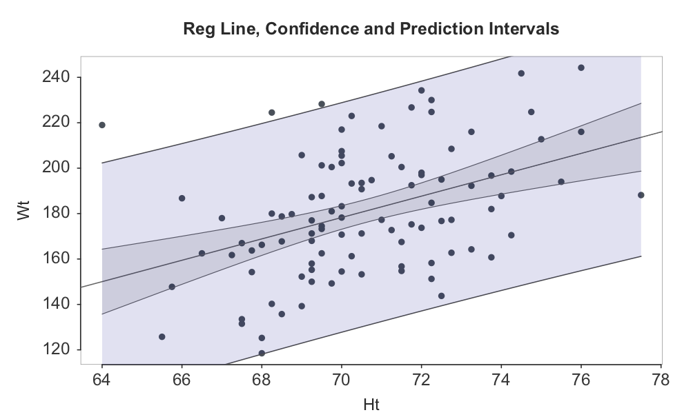
For that, we need the prediction interval, about plus or minus about two standard errors of prediction. Figure 4.7 shows the prediction interval for all the values of X, here Ht, in the analysis. The area between the inner curved lines that enclose the darker shaded area indicates the typical variation of the sample regression line from sample to sample, reflecting sampling error only. The area between the outer curved lines indicates the typical fluctuation of the predicted values from sample to sample, the prediction intervals, which reflect both training error and sampling error. Here shown for \(n=100\) to include more detail and more representative visualization than obtained from only \(n=10\).
4.3.4 Example
4.3.4.1 Computer Analysis
As an example, we return to our simple Ht-Wt analysis. Obtain prediction intervals for two different heights, neither of which are in the original data table: 67.5 inches and 71.0 inches. The prediction interval output and explanation of the included symbols follows. The model was previously estimated as
\[\hat y_{w} = -393.788 + 8.520(x_{h})\] Here, re-estimate the model and also calculate the prediction with its associated prediction interval for values of Height of \(67.5\) and \(71.0\) inches.
----------------------------------------------------
        Ht  Wt    pred s_pred  pi.lwr  pi.upr  width
  1 67.500     157.656 15.148 122.725 192.587 69.862
2 71.000 175.861 14.420 142.608 209.114 66.506- Ht: x-variable value
- Wt: y-variable value; missing because it is unknown, a true prediction
- pred: predicted value, \(\hat Y_i\)
- s_pred: standard error of prediction
- pi.lwr: lower bound of 95% prediction interval
- pi.upr: upper bound of 95% prediction interval
- width: width of the 95% prediction interval
☞ Show the calculation of the fitted/predicted value of Weight for the value of predictor variable \(X_{h}=67.5\) inches.
\[\begin{align*}
\hat y_{w} &= -393.788 + 8.520(x_{h})\\
&= -393.788 + 8.520(67.5)=157.66
\end{align*}\]
The value of the predicted weight for someone \(67.5\) inches tall is \(157.66\) lbs.
Unfortunately, the specific predicted value is almost certainly wrong.
For a person \(67\) inches tall, their weight will almost never be the predicted \(157.66\) lbs. It might, and hopefully is, close to \(157.66\) lbs, but it will generally not be that value.
A viable prediction is a range of values that likely contains the actual value when becomes known.
From the computer output, for an adult male with a height of \(67.5\) inches, the corresponding prediction interval is \(122.7\) to \(192.6\) lbs. Note that this is the prediction interval, not its interpretation, provided below.
4.3.4.2 Manual Construction
We can manually construct to illustrate the underlying concept, which, given the computationally intensive standard error of prediction, \(s_{pred}\), is straightforwardly computed. To build the prediction interval, we need the 95% range of variation of the predicted value under repeated sampling. Assuming a normal distribution, that range would be 1.96 standard deviations, here the standard error of prediction, \(s_{pred}\).
Because we have to estimate this standard error, use the corresponding \(t\)-distribution in place of the normal distribution, which provides a wider interval than from the normal curve 1.96 cutoff. The \(t\)-cutoff for an hypothesis test with \(\alpha = 0.05\) is \(t_{0.25} \approx 2\). For small samples such as this \(n=10\), \(t_{0.25}\) is larger, \(2.306\).
Obtain the exact value from the \(t\)-probability function. The degrees of freedom is \(n-2\), based on first estimating \(b_0\) and \(b_1\), then returning to the same data and calculating the deviation scores (errors) from the model defined by these estimates. Use the lessR function prob_tcut() to get the exact value of \(t_{0.25}\).
n <- 10
prob_tcut(n-2)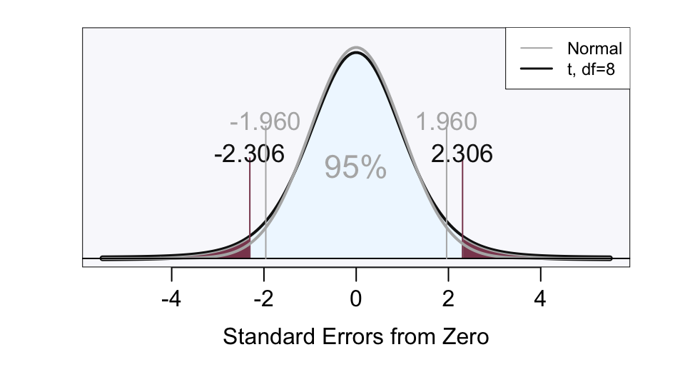
Probability: 2.306004 Compute the prediction interval for a predicted value, as with a confidence interval of a statistic, from the corresponding margin of error. The standard error of prediction for each individual value of \(x\) changes depending on the value of \(x\). Here, for someone with a height of 67.5 inches, \(s_{pred}\) is 15.148.
☞ For the 95% prediction interval of Weight for the value of predictor variable Height of 67.5, show the interval including its calculation (can approximate with the \(t\)-cutoff of 2 but here use the actual \(t\)-cutoff).
\(E = (t_{.025})(s_{\hat y_{67.5}}) = (2.306)(15.148) = 34.93\)
From the margin of error, E, get the prediction interval.
\[\textrm{lower bound: } \hat y - E = 157.66 - 34.93 = 122.7\] \[\textrm{upper bound: } \hat y + E = 157.66 + 34.93 = 192.6\]
Our prediction, then, is not a single value, but a range of values, from \(122.7\) to \(192.6\) in this example.
4.3.4.3 Interpretation
The interpretation of any statistical output is free of statistical jargon, as it would be explained to management or to the client, whoever sponsored the analysis. The interpretation is the reason why the analysis was conducted.
☞ Interpret the prediction interval.
For an adult male who is 67.5 inches tall, with 95% confidence, the weight for that person is predicted to be somewhere within the range from 122.7 lbs to 192.6 lbs.
The prediction interval is almost \(70\) lbs wide. This prediction interval is so wide as to render the prediction meaningless. This dismal precision level is not surprising given the small sample size and wide variability of the data around each point on the regression line.
The prediction interval communicates the precision of the prediction.
A single predicted value can always be obtained, in this case, \(\hat y\) = 157.66 lbs for a height of 67.5 inches. But the actual value of \(y\) when obtained would not equal exactly its predicted value, \(\hat y\). Analysis of the size of the prediction interval provides the actual prediction. We are close to 0% of being correct for the specific predicted value. Given the assumptions of our model and sampling procedure, we have a 95% confidence level of being correct that the actual value will be within the prediction interval.
We saw that the standard error of prediction consists of the respective contributions of:
- Training (modeling) error, \(s_e\), the standard deviation of the residuals about the regression line
- Sampling error, \(s_{\hat y_{p,i}}\), the standard deviation of a point on the regression line over repeated sampling
To decrease the width of the prediction intervals:
- Decrease training error by improving the model, such as by adding additional predictor variables or adjusting for non-linearities
- Decrease sampling error by increasing sample size
The goal in forecasting is always to decrease the width of the prediction intervals as much as possible to obtain more precise predictions.