
11.1 Overview
Logistic regression is the classic and historically earlier classification procedure. Modern machine learning, however, provides many alternatives in the pursuit of greater predictive accuracy. With modern computing power, analysts can compare different estimation algorithms, model structures, and parameter settings, even for large data sets.
Another widely used classification procedure is the decision tree. Like logistic regression, a decision tree can be applied to a categorical target variable with two or more classes, also called labels, levels, values, or groups. Unlike logistic regression, a decision tree produces a sequence of decisions that leads to a final classification.
Decision tree: A hierarchical structure of binary decisions used to predict the class of an observation.
The process begins with all the data in a single group. The tree then repeatedly divides the observations into smaller and increasingly homogeneous groups, meaning that the observations within each resulting group tend to belong to the same target class.
Each binary decision is typically based on a cutoff value for a feature variable. Observations with values on one side of the cutoff are assigned to one branch of the tree, while observations with values on the other side are assigned to the second branch.
For example, consider the amount of credit-card debt expressed as a percentage of income. A decision tree might first divide bank customers according to whether their debt-to-income percentage is above or below a particular threshold. Customers above the threshold would follow one branch of the tree, and customers below the threshold would follow the other.
In practice, a lending decision would usually depend on several variables rather than on a single threshold. After the first split, the tree can introduce additional decisions based on the same feature or on other features, such as income, credit history, or employment status. The resulting sequence of questions can be expressed as If–Then rules. Following these rules from the top of the tree to a final endpoint assigns each observation to a predicted class, such as approving or rejecting a loan application.
11.2 Example
To illustrate how a decision tree is constructed, return to the data from an online clothing retailer that predicts whether a customer is a man or a woman from physical measurements. Consider a simplified analysis based on only two features: hand size and height. Figure 11.1 displays a scatterplot for 340 actual customers, with the measurements for men and women shown in different colors. Use this scatterplot to explore the possibility of predicting gender from these two body measurements.
Because height and hand size take on a limited number of recorded values, multiple observations can appear at the same location in the scatterplot. Plot the points with partial transparency to reduce this overplotting. Transparency does not fully resolve the issue, however, because points from different groups can occupy the same coordinate, and multiple points of the same color may appear as a single point. Consequently, the exact number of observations at some locations cannot be determined from the graph. Even so, the plot provides a useful visual guide to how a decision tree defines regions containing increasingly homogeneous groups of observations.
According to Figure 11.1, classification from these measurements appears feasible because the measurements for men and women generally cluster in different regions of the scatterplot. Men tend to appear toward the upper-right, whereas women tend to appear toward the lower-left. The groups overlap, so perfect classification is not possible from these two features alone, but the visible separation suggests that a classification algorithm should be able to predict many observations successfully.
The decision tree algorithm begins by considering all observations together. It then evaluates possible splits based on the available features and selects the split that produces the greatest improvement in class homogeneity. For this application, a useful split would create one group containing a relatively high proportion of men and another group containing a relatively high proportion of women.
At each step in constructing the tree, evaluate the proposed splits with an impurity measure. A node is perfectly homogeneous, or pure, when all observations in that node belong to the same class, such as all Male or all Female.
Gini impurity (for a decision tree): An index of the extent to which the classes are mixed within a node. A value of 0 indicates perfect homogeneity because every observation belongs to the same class. Larger values indicate greater mixing of the classes.
The closer the Gini impurity is to zero, the more homogeneous the node. For a binary target, the maximum Gini impurity is 0.5, which occurs when the two classes are equally represented. For example, as shown in Figure 11.3, the initial, or root, node contains 170 females and 170 males and therefore has a Gini impurity of 0.5.
For example, to classify a customer as a man or a woman from physical dimensions such as hand size and height, the tree might first divide all customers according to whether hand size is above or below a selected cutoff value. Within each of the resulting groups, the tree can then make another split based on height, hand size again, or another available feature. Each successive split produces smaller and generally more homogeneous groups.
The ideal result, rarely obtained with real data, would be a sequence of decisions that ends in groups containing only male body types or only female body types. Such terminal groups would be perfectly homogeneous. In practice, however, allowing the tree to continue splitting until nearly every training observation is classified correctly can overfit the model to the particular data used for estimation.
Gini impurity is the default criterion used by Python’s sklearn DecisionTreeClassifier to evaluate potential splits. At each node, the algorithm considers possible feature and cutoff combinations and selects the split that produces the largest weighted reduction in Gini impurity across the resulting child nodes. (Scikit-learn)
Although the tree is constructed by repeatedly reducing impurity, evaluate the predictive performance of the completed model on separate test or validation data. For a classification model, this evaluation includes the confusion matrix and its counts of true positives, true negatives, false positives, and false negatives, as discussed below.
11.2.1 Split #1
For a given data set, the decision tree algorithm examines the available features one at a time. For each feature, it evaluates possible cutoff values and identifies the cutoff that produces the most homogeneous resulting groups.
Decision boundary: A cutoff value for a feature that divides the observations into two subsets.
After evaluating the possible splits across all features, the algorithm selects the single feature-and-cutoff combination that produces the greatest reduction in impurity.
For these data, hand size provides the best first split. The decision tree algorithm identifies the following decision boundary:
- Hand size < 8.125
- Hand size \(\geq\) 8.125
The observations with hand size below 8.125 are predominantly female, whereas those with hand size at least 8.125 are predominantly male. A decision tree limited to this single split therefore provides a simple prediction rule: predict Female when hand size is less than 8.125 and predict Male otherwise.
The first split is derived from the root node, which contains all observations in the training data.
Root node: The node at the top of the inverted tree that contains all observations before the first split.
The basis for the chosen split is illustrated in Figure 11.2. The vertical decision boundary at a hand size of 8.125 separates the two classes as effectively as possible for the first split. Most of the male observations appear to the right of the boundary, whereas most of the female observations appear to the left. Because the classes still overlap, however, this single split does not classify every observation correctly.

The resulting output for this single binary split at a hand circumference of 8.125 inches appears in Figure 11.3. The root node contains all 340 samples: 170 females and 170 males. Because the two classes are equally represented, the root node has a Gini impurity of 0.5.
Each node displays the class that the model would predict for an observation that ended at that node. This simple decision tree has a maximum depth of 1. Consequently, the two nodes created by the first split are terminal nodes, or leaves, because the tree makes no further divisions.
At the root node, the estimated probabilities of Female and Male are both 0.50. When two classes have the same highest estimated probability, DecisionTreeClassifier predicts the class with the lower position in its classes_ attribute. Here, Female precedes Male in the ordering of the class labels, so the displayed prediction at the root is Female. This prediction is only the class associated with that node; it does not designate Female as a “True” value for the subsequent split.
This class ordering should also not be interpreted as defining a reference group. Unlike logistic regression, a decision tree does not require one target class to be omitted as a reference category. It uses all target classes directly when evaluating splits and making predictions.
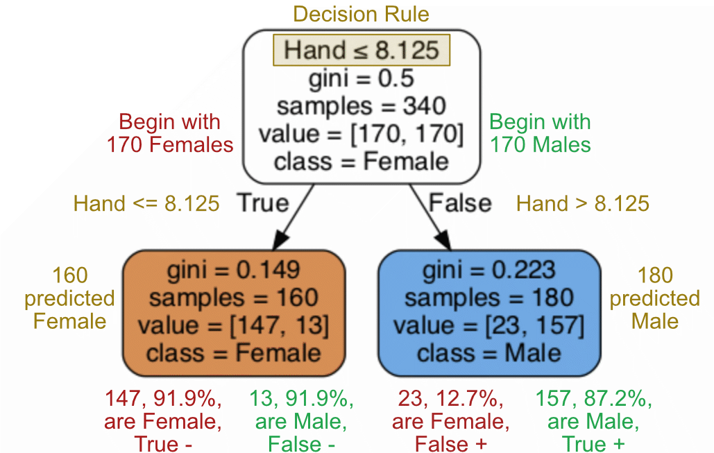
Interpret a decision tree, such as the tree in Figure 11.3, according to the following rules.
The decision rule appears at the top of each internal node—that is, each node that produces another split. The rule compares the value of one feature with a specified cutoff value.
A leaf, or terminal node, does not contain another decision rule. Instead, it represents the final predicted class for observations that reach that node. Although leaves often appear along the bottom of a simple tree, an unbalanced tree can contain leaves at different depths.
If an observation satisfies the decision rule at a node, follow the left branch. Otherwise, follow the right branch. For example, a rule written as
Hand <= 8.125sends observations satisfying that condition to the left and all remaining observations to the right.Read
class =as predicted class =. It indicates the class the model would predict for an observation that ended at that node.The predicted class at a node is generally the class containing the largest number of training observations at that node. If two classes have equal counts, the algorithm resolves the tie according to the ordering of the class labels.
The entries in
valuereport the number of observations from each actual class at that node. Their order follows the class labels stored in the fitted model’sclasses_attribute. For example, if the class order is Female followed by Male,value = [120, 20]indicates 120 females and 20 males.The values in the leaves can be used to construct a confusion matrix. Each leaf provides the actual class counts for observations assigned the predicted class shown for that leaf. After designating one class as the positive class, combine these counts across the leaves to obtain the true positives, true negatives, false positives, and false negatives.
The color of each node represents its predicted class, and the intensity of the color represents the purity of that node. A more saturated color indicates that a larger proportion of the observations belong to the predicted class and, correspondingly, that the Gini impurity is lower.
How accurate are the predictions from this simple decision tree with only one decision rule? The confusion matrix in Table 11.1 follows from the class counts in the two leaves of Figure 11.3. Each observation is assigned the predicted class of the leaf it reaches, and the actual class counts within those leaves determine the four entries of the confusion matrix.
| actual | pred F | pred M |
| F | 147 | 23 |
| M | 13 | 157 |
The first split at a hand circumference of 8.125 inches produces a group predicted as Female that contains 147 females and 13 misclassified males. The group predicted as Male contains 157 males and 23 misclassified females. This single-split decision tree therefore achieves a classification accuracy of 89.4%.
\[\mathrm{Accuracy}=\frac{\text{true positives}+\text{true negatives}} {\text{all observations}} = \frac{147+157}{147+13+157+23} = 0.894\]
Will additional model complexity improve predictive accuracy? A decision tree becomes more complex by adding further splits below one or more of the existing nodes. At each node, the algorithm evaluates the available features and cutoff values and introduces another split only when doing so sufficiently reduces impurity, subject to the model’s stopping rules.
11.2.2 Split #2
The first split in the decision tree shown in Figure 11.3 partitions the complete data set into two groups. In Figure 11.2, these groups are represented by the observations to the left and right of the vertical decision boundary.
This first split produces a tree with a depth of 1.
Tree depth: The maximum number of decision rules encountered along a path from the root node to a leaf.
To obtain a more complex model with a depth of 2, apply the same splitting logic within each of the two partitions created by the first split. For each partition, the algorithm again evaluates the available features and cutoff values and selects the split that most reduces Gini impurity.
First, consider the partition to the left of the vertical boundary in Figure 11.2, which contains the observations initially predicted as Female. Within this partition, where should a horizontal decision boundary based on height be placed to produce the most homogeneous resulting groups? The lower portion contains mostly blue points, representing females, whereas the upper portion contains a larger proportion of brown points, representing males. Figure 11.4 displays the resulting horizontal boundary at a height of 69.5 inches.

Next, apply the same logic to the partition to the right of the vertical boundary in Figure 11.2 and Figure 11.4. Within this mostly male group, the most effective height boundary is lower than the boundary for the first partition. Placing the split at 65.5 inches better separates the blue points near the bottom from the predominantly brown points above. Figure 11.5 illustrates this second conditional decision boundary.

These partitions produce the decision tree with a depth of 2 shown in Figure 11.6. As before, less saturated node colors indicate a larger proportion of observations from the class not predicted at that node and, therefore, greater impurity.
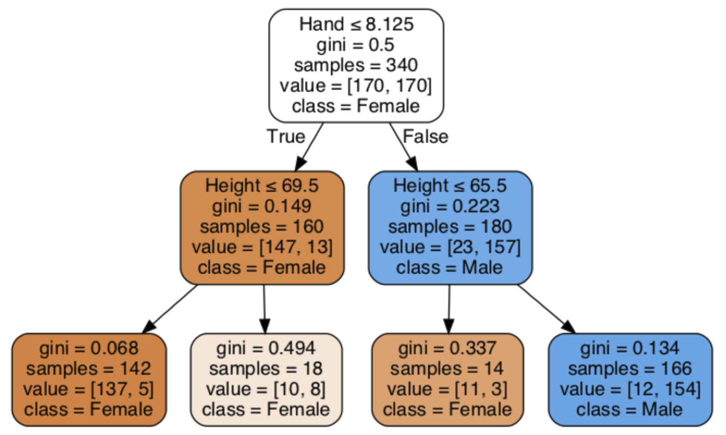
At depth 2, only the leaf on the far right predicts Male. Reaching this leaf requires satisfying two sequential decision rules. First, the customer must have a hand size of at least 8.125 inches, which sends the observation to the right branch of the root node. Of the 180 customers in this partition, the 166 with a height greater than 65.5 inches then follow the right branch of the second decision and receive a final prediction of Male.
Leaf: A terminal node that makes no further split and provides the final predicted class for observations that reach it.
The remaining three leaves predict Female. Of all four leaves, the leaf at the far left of Figure 11.6 has the smallest percentage of misclassified observations. It contains customers with a hand size less than or equal to 8.125 inches and a height less than or equal to 69.5 inches. Of the 142 customers who satisfy these two conditions, 137 are correctly classified as Female and 5 are misclassified males. Accordingly, this leaf has the lowest Gini impurity, 0.068.
The leaf second from the left in Figure 11.6, corresponding to the upper-left partition in Figure 11.5, provides the least accurate classification. Customers with a hand size less than or equal to 8.125 inches but a height greater than 69.5 inches are almost evenly divided between the two classes. The slight majority of 10 females compared with 8 males results in a prediction of Female for customers who reach this leaf.
From a decision-making perspective, the organization might choose not to assign a gender prediction when the estimated classification is this uncertain. Instead, the system could return a result such as Undecided. The machine learning analyst could also investigate whether additional body measurements provide enough information to distinguish more reliably between males and females in this subgroup.
The correct and incorrect classifications in the four leaves of Figure 11.6 provide the counts needed to construct the confusion matrix. Across the three leaves that predict Female, the numbers of misclassified males are 5, 8, and 3, for a total of 16 males incorrectly predicted as Female. The single leaf that predicts Male contains 12 females incorrectly predicted as Male. Table 11.2 presents the complete confusion matrix.
| actual | pred F | pred M |
| F | 158 | 12 |
| M | 16 | 154 |
From the confusion matrix, the computation of accuracy quickly follows.
\[ \mathrm{accuracy=\frac{true \; positives + true \; negatives}{all \; outcomes}=\frac{158 + 154}{158+16+154+12}=0.918}\]
The second level of splits increased classification accuracy from 89.4% to 91.8%, an improvement of 2.4 percentage points. Will adding a third level produce a similar improvement?
11.2.3 Split #3
At the third level of the tree, the algorithm can return to hand size and use a different cutoff to further divide one or more of the four existing partitions. A decision tree may use the same feature more than once because each split is evaluated only within the subset of observations that reaches that node.
Focus on the upper-left partition in Figure 11.5, which contains 10 females and 8 males. Because these observations are nearly evenly divided between the two classes, the prediction of Female at this node is relatively uncertain. The decision tree therefore evaluates whether another split can produce more homogeneous groups. Figure 11.7 shows the additional partition based on hand size at the third level.

Further considering hand size, the algorithm separates the three females whose hand size is less than 7.75 inches. The resulting new leaf at the third level contains three observations, all correctly classified as Female.
The remaining uncertainty lies among the other 15 customers from the original partition: seven females and eight males. This nearly even division appears in the tree diagram in Figure 11.8 and in the corresponding shaded region of Figure 11.7. These observations represent relatively tall customers whose hand sizes fall within the narrow interval between 7.75 and 8.125 inches.
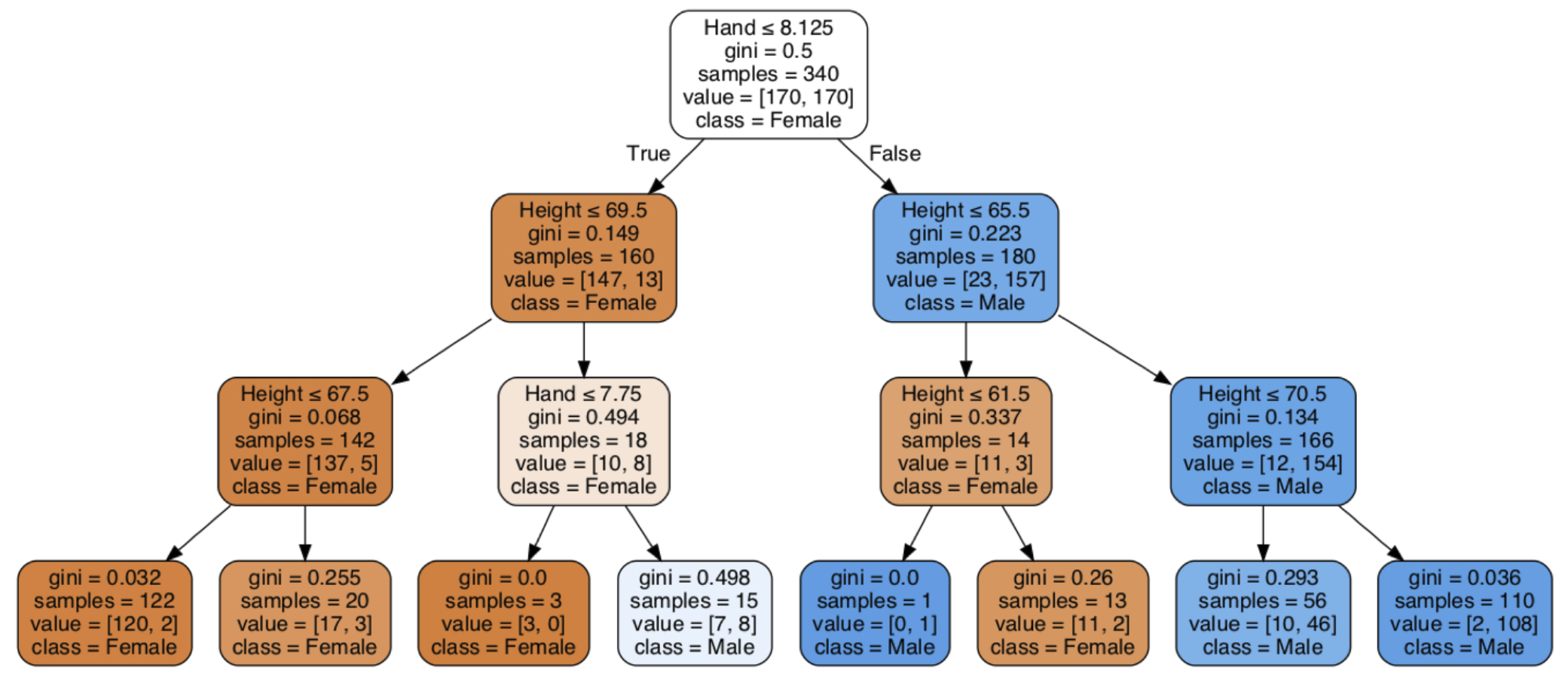
Construct the confusion matrix from the class counts in the terminal leaves of Figure 11.8. A tree with a depth of 3 can have as many as (2^3=8) leaves, but only when every eligible node splits at each level. The actual number of leaves depends on which nodes the fitted tree divides.
With Male designated as the positive class, a female predicted as Male is a false positive. The three Male-predicting leaves on the right contain a total of 12 misclassified females. The additional leaf containing seven females and eight males also predicts Male and so contributes seven more false positives, for a total of 19.
Table 11.3 presents the complete confusion matrix for evaluating the decision tree with a depth of 3.
| actual | pred F | pred M |
| F | 151 | 19 |
| M | 7 | 163 |
Computation accuracy as follows.
\[ \mathrm{accuracy=\frac{true \; positives + true \; negatives}{all \; outcomes}=\frac{163 + 151}{163+7+151+19}=0.924}\]
Accuracy increases only slightly from 0.918 for the depth-2 tree to 0.924 for the depth-3 tree, an increase of 0.006, or 0.6 percentage points. The additional split also changes the types of classification errors. With Male designated as the positive class, the number of false negatives decreases from 16 to 7, so sensitivity, or recall, increases. However, the number of false positives increases from 12 to 19, which reduces precision and specificity.
Consequently, the depth-2 tree would be preferred when avoiding false-positive Male classifications and maintaining a simpler, more interpretable model are more important than the small improvement in overall accuracy and sensitivity. The depth-3 tree might instead be preferred when failing to identify a male customer carries the greater cost.
The decision tree in Figure 11.8 also reveals substantial variation in classification accuracy across its leaves. Among customers with a hand size greater than 8.125 inches and a height greater than 70.5 inches, 108 of 110 are correctly classified as Male. This leaf therefore has a Gini impurity close to zero, 0.036. For this sample, its classification accuracy is
\[\frac{108}{110}=0.982\]
or 98.2%.
In contrast, consider the pale-colored leaf in which males and females are least well distinguished. Its Gini impurity is 0.498, close to the maximum of 0.5 for a binary target. The customers in this leaf have hand sizes less than or equal to 8.125 inches but greater than 7.75 inches. They are also taller than 69.5 inches. The leaf contains seven females and eight males, so the two classes are almost evenly represented.
Customers with relatively tall heights but hand sizes just below the original cutoff of 8.125 inches are therefore difficult to classify as Male or Female using only these two measurements. Additional body measurements might provide the information needed to distinguish these customers more reliably.
11.3 Overfitting
The decision tree with a depth of 3 improved accuracy only slightly over the depth-2 tree. What happens as additional levels are added and the model becomes increasingly complex? Greater complexity may continue to improve the fit to the training data, but it does not necessarily improve prediction for new observations.
As discussed in Section Section 4.1.4 on prediction error, a model can fit the training data too closely. In that case, the estimated model overfits the data. As a decision tree grows deeper, it gains more opportunities to create increasingly narrow partitions that account for the particular combinations of hand size, height, and gender found in the training sample.
With sufficient complexity, a model can achieve nearly perfect prediction on the training data by modeling idiosyncratic sampling variation rather than relationships that generalize to new data.
Perfect classification of the training observations has little practical value by itself because the model was estimated from data for which the correct classifications were already known. The more important question is how accurately the fitted tree classifies observations that were not used to estimate it.
What happens when the maximum depth of the decision tree for predicting Gender increases to 10? The result is an overfit model, as shown by the following 5-fold cross-validation results. For each fold, fit the model on four-fifths of the observations and evaluate it on the remaining one-fifth.
The training accuracy, reported in the train_accuracy column, is 1.000 for every fold. The depth-10 tree perfectly classifies all males and females in each training sample.
The validation accuracy, reported in the test_accuracy column, tells a different story. Its average across the five folds is 0.891, which is lower than the corresponding average of 0.921 for the depth-2 tree. Increasing the maximum depth from 2 to 10 therefore improves training fit but worsens predictive performance on observations not used to estimate the model.
This pattern—near-perfect training accuracy accompanied by lower validation accuracy—is evidence of overfitting.
   fit_time  score_time  test_accuracy  train_accuracy  test_recall  \
0     0.004       0.009          0.882             1.0        0.889
1     0.003       0.004          0.882             1.0        0.842
2     0.004       0.006          0.941             1.0        0.933
3     0.002       0.004          0.897             1.0        0.889
4     0.002       0.004          0.853             1.0        0.833

   train_recall  test_precision  train_precision
0           1.0           0.889              1.0
1           1.0           0.941              1.0
2           1.0           0.933              1.0
3           1.0           0.914              1.0
4           1.0           0.833              1.0
` Although overfitting from an overly complex model is the more common concern, consider the opposite problem: underfitting. In this example, the decision tree with a depth of 1 performs worse on the validation data than the tree with a depth of 2. The depth-1 model is too simple to capture enough of the relationship between the predictor variables and Gender.
A central challenge in machine learning is to find the appropriate balance between underfitting and overfitting. A model that is too simple fails to capture important structure in the data, whereas a model that is too complex begins to model random variation specific to the training sample. The preferred model achieves parsimony: it is as simple as possible without sacrificing meaningful predictive performance, but no simpler. See Section Section 4.1.4 and Figure 4.1 for a more extensive discussion and illustration of this balance.
11.4 Hyperparameter Tuning
11.4.1 Parameter vs. Hyperparameter
Parameters are learned; hyperparameters are chosen.
What does the machine learn in an application of machine learning? The selected estimation algorithm uses the training data to estimate the values of the model’s parameters. These parameters define the specific fitted model.
For a linear model, the parameters include the intercept and the coefficient, or weight, assigned to each feature, such as the (b_i) values. For a decision tree, the learned parameters include the selected features, cutoff values, and resulting tree structure.
Model parameter: A quantity estimated from the training data that defines a specific fitted model.
Fitting a linear model estimates the intercept and slope coefficients used to predict (y). Fitting a decision tree determines the sequence of feature-based splits that leads to a predicted value or class of (y).
Other characteristics of the model are specified by the analyst before the estimation process begins.
Hyperparameter: A model setting specified before training that guides how the learning algorithm constructs the fitted model.
Hyperparameters for a decision tree include the maximum tree depth, the minimum number of observations required to create a split, and the number of features considered when evaluating a split. A maximum depth of 4, for example, defines a different possible model structure than a maximum depth of 5.
For each selected set of hyperparameter values, the learning algorithm fits a new model and estimates its parameters from the training data. The resulting models can then be compared according to their performance on validation data.
Hyperparameter tuning: Evaluate alternative values of model settings specified before estimation and select the combination that provides the best validation performance.
A grid search provides one systematic approach to hyperparameter tuning. The analyst first defines a set of possible values for each hyperparameter. The procedure then fits and evaluates a model for each specified combination of values. Comparing the resulting validation scores helps identify the model structure that provides the best balance of predictive performance and complexity.
11.4.2 Grid Search
The Python sklearn framework provides a formal procedure for systematically comparing a set of related models. Instead of fitting only one model configuration, the analyst specifies several possible values for selected hyperparameters and evaluates the predictive performance of every combination in that predefined set.
For example, how does classification accuracy change when maximum tree depth increases from 3 to 4? Does considering five features at each split improve prediction compared with considering only three? Grid search addresses such questions by fitting and evaluating a separate model for each specified combination of hyperparameter values.
Grid search: Evaluate a predefined set of hyperparameter combinations and compare the predictive performance of the resulting models.
Adding grid search to a supervised machine learning analysis produces the following general progression:
- Especially when a large data set or complex algorithm requires substantial computing time, begin with a single training–test split to determine whether the modeling approach appears promising.
- If the approach is promising, evaluate a specific model configuration more reliably with (k)-fold cross-validation.
- Extend the analysis beyond a single model configuration by using grid search. Evaluate each specified combination of hyperparameter values with its own (k)-fold cross-validation.
The primary cost of grid search is computing time. Suppose two hyperparameters each have five candidate values. The grid contains
\[5 \times 5 = 25\]
hyperparameter combinations. If each combination is evaluated with 5-fold cross-validation, the procedure fits
\[5 \times 5 \times 5 = 125\]
models. After comparing the average validation performance across the 25 configurations, select the combination that provides the preferred balance between predictive performance and model parsimony.
The purpose of this procedure is to choose a model configuration that is expected to predict new observations accurately. However, repeatedly examining performance on the same test data would gradually adapt the modeling decisions to that test set. The test data would then no longer provide an independent evaluation of the final model.
A more appropriate procedure separates model selection from final model evaluation. Use the training data and cross-validation folds to tune the hyperparameters. After choosing the preferred hyperparameter values, evaluate the resulting model once on a separate test set that was not used during tuning.
Data leakage: Information outside the training data improperly influences model estimation or model selection, producing an overly optimistic assessment of predictive performance.
The most obvious form of data leakage occurs when a model is evaluated on the same observations used to fit it. More subtle leakage can occur during data preprocessing. For example, calculating the mean and standard deviation from the entire data set before creating the training and test sets allows information from the test observations to influence the standardized training data.
Instead, fit the standardization procedure using only the training data. Then use the training-data means and standard deviations to transform both the training data and the test data. During (k)-fold cross-validation, repeat this process within each fold: fit the transformation on that fold’s training portion and apply it to the corresponding validation portion. An sklearn pipeline provides a convenient way to enforce this separation.
The good news is that if we avoid data leakage, we can “fish” as much as we wish because any chance optimization on the training data by definition does not generalize to testing data. To our benefit, sklearn makes this fishing expedition easy. The application of machine learning does not apply newly discovered laws of statistics. Instead, it relies upon access to modern computing power and large data sets to accomplish analyses that were either impossible or impractical in earlier times.
11.4.3 Three-Way Data Splits
As always, evaluate a fitted model on data not used for its estimation to assess how well it generalizes to new observations. Hyperparameter tuning introduces an additional complication because multiple model configurations are fitted and compared. If all configurations are evaluated on what was originally called the test set, and the best configuration is selected from those results, the test set has influenced model selection. It can no longer provide an unbiased estimate of final predictive performance.
For this reason, model selection ideally uses three data subsets rather than only the usual training and test sets. This arrangement is called a training–validation–test split.
With hyperparameters, ideally follow this three-step process:
- Training data: Fit multiple models using different combinations of hyperparameter values.
- Validation data: Evaluate the fitted models and select the hyperparameter combination that provides the best validation performance.
- Test data: Evaluate the final selected model once on the test set to obtain an unbiased estimate of generalization to new data.
After selecting the hyperparameters, the analyst commonly refits the model using the combined training and validation data. The model is then evaluated once on the untouched test data.
Once model choices are adjusted in response to performance on a particular data set, that data set is no longer an independent test set. It has become part of the model-selection process and therefore serves as validation data. The more often the analyst examines the results and revises the model accordingly, the more the model-selection process becomes adapted to that data, as illustrated in Figure 11.9.

After selecting the hyperparameter values from validation performance, evaluate predictive accuracy on the test data, which must remain completely separate from model fitting and model selection. The test set should be examined only after the final model configuration has been chosen.
Without a separate validation process, repeatedly comparing hyperparameter values on the test set would allow information from the test data to influence the chosen model. This practice would not necessarily constitute direct leakage into model fitting, but it would produce an overly optimistic estimate of generalization because the test set would no longer be truly independent.
The division of labor among the three data sets matters, and it is easy to compromise without noticing. The training data fit each model. The validation data select among models and settings, whether choosing a learning rate, deciding the number of boosting rounds through early stopping, or determining which of the four methods to carry forward. The test data are used once, at the end, to report how well the selected model performs. A test set consulted repeatedly while models are compared has become a second validation set, and the accuracy it reports is no longer an honest estimate, because the model was chosen partly on the basis of that very result.
A three-way split requires enough observations for each of the training, validation, and test subsets to be large enough to serve its purpose. When the available data are more limited, cross-validation within the training data can take the place of a separate validation set, while a test set is still preserved for the final evaluation. Cross-validation serves two distinct purposes, and keeping them separate clarifies what the procedure accomplishes. The first purpose is to estimate how well one particular model predicts. Rather than relying on a single hold-out sample, \(k\)-fold cross-validation divides the training data into \(k\) folds and fits the model \(k\) times, each time withholding a different fold and evaluating the fitted model on the observations withheld. Each fold acts as a validation set in turn, and the \(k\) results are averaged into a single estimate of predictive accuracy. The averaging is the point. A single hold-out sample yields an estimate that depends on which observations happened to fall into it, whereas averaging across \(k\) different hold-out samples yields a more stable estimate. Nothing is being compared here because only one model is being evaluated.
The second purpose is to choose among competing models, which ordinarily means choosing among combinations of hyperparameter values. The entire \(k\)-fold procedure just described is then carried out separately for each candidate. A search over three learning rates and four tree depths, for example, defines twelve candidate models, and each of the twelve is cross-validated in full, producing twelve averaged accuracy estimates that can be compared on equal terms. The candidate with the best estimate is selected.
The two purposes are nested. The folds form the inner loop, which evaluates a single model. The candidates form the outer loop compares many models. A run of twelve candidates with five folds fits sixty models altogether, which is why a large search over hyperparameter values be comes computationally demanding.
The distinction also explains why a test set remains necessary. Used for the first purpose alone, on a model specified in advance, cross-validation gives an honest estimate of that model’s accuracy. Used for the second, the winning candidate was chosen precisely because it achieved the best cross-validated score, so that score is optimistic as a description of the model finally selected. The final evaluation belongs to the test set, which took part in neither loop.
11.5 Summary
A decision tree classifies an observation by following a sequence of feature-based decisions from the root node to a terminal leaf. At each node, the algorithm chooses the feature and cutoff value that most reduces class impurity in the resulting groups. The completed tree can then be interpreted as a set of If–Then rules.
Tree depth controls model complexity. A shallow tree may underfit the data by failing to capture important structure, whereas a deep tree may overfit by modeling random variation in the training sample. For this reason, evaluate predictive performance on data not used to estimate the model rather than relying only on training accuracy.
Hyperparameters such as maximum tree depth, minimum observations required for a split, and the number of features considered at each node determine the range of tree structures the algorithm may construct. Grid search and cross-validation provide a systematic way to compare these settings while limiting overfitting during model selection. A separate test set should remain untouched until the final model configuration has been chosen.
Decision trees are attractive because their predictions can be represented as understandable decision rules. A single tree, however, can also be unstable: relatively small changes in the training data may produce different splits and a different tree structure. The next chapter addresses this limitation by combining many decision trees into ensemble models. Random forests use repeated samples and multiple trees to stabilize predictions, while boosting methods such as XGBoost build trees sequentially to improve the errors that remain.