| Veggies | ChipsEtc |
|---|---|
| 2.86 | 4.59 |
| 2.50 | 7.01 |
| 4.50 | 1.71 |
| 7.74 | 2.81 |
| 2.26 | 4.09 |
| 8.89 | 2.34 |
| 6.48 | 3.68 |
| 1.62 | 4.47 |
12.1 Overview
The search for patterns with or without a target variable distinguishes between supervised and unsupervised machine learning. With supervised learning the target values guide, that is, supervise, the machine (solution algorithm). From the provided examples, the data, the machine develops predictive equations that associate the information provided by the predictor variables (features) with the target from the provided examples.
Labeled dataset: Data contains examples of the target value associated with values of the features.
Supervised machine learning teaches the machine to emulate the values of the associated target values from the features.
How to proceed without a target variable? Unsupervised learning uncovers structure inherent in the data.
Unsupervised machine learning: Recognize patterns without identifying a target variable.
Unsupervised learning identifies patterns of examples, such as consumers, that have similar values on the features.
12.1.1 Cluster Analysis
The primary form of unsupervised learning is cluster analysis, which identifies groups of similar samples.
Cluster analysis: Identify groups (clusters) of samples (examples, instances, observations) with similar values on the feature variables, and dissimilar values with samples in other groups.
A classic application of cluster analysis is market segmentation, which classifies consumers according to income and demographic characteristics. Another application is the grouping of shopping cart contents such as at a grocery store, identifying products that tend to be purchased together. Or, identify groups of products with high sales and revenues at specific locations to more optimize warehousing of inventory.
Discovering the group structure reveals the key variables by which the data are organized. This information can then, in turn, form the basis for a targeted classification model, in which additional samples are classified into the discovered groups. Or, this structure may be further developed such as with logistic regression or decision trees in which new samples are classified into the corresponding group.
How to form the groups, that is, clusters? Express similarity of the values on the feature variables in terms of distance. The average distance of samples (objects, points) within a cluster should be as small as possible, and the average distance between clusters should be larger. Cluster analysis, then, is the analysis of distances.
12.1.2 Example
Consider a shopping cart example, data which are now so readily available to grocery chains given that all items are now scanned at the check-out counter. Suppose that two types of shoppers have been identified, named Healthy Food customers and Junk Food customers, here with contrived, simplistic data for illustration. The amount spent on two categories of food is recorded for each customer, Fresh Vegetables and foods such as Chips, shown in Table 12.1.
The data for each shopper are averaged over many shopping trips. Otherwise, someone who bought primarily veggies one trip may already have many chips and similar at home, and on the next trip buy many more chips. Only averages of each variable over many trips would provide a reliable response needed to properly characterize customers by their shopping patterns.
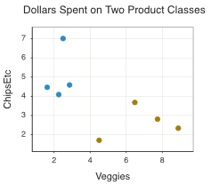
A quick glance at the data shows that customers who tend to favor the chips etc. do not buy many fresh vegetables. And, those who favor the vegetables buy less food such as chips. To further understand this pattern, the data for an analysis with just two features can be plotted in two dimensions, one dimension for each feature.
The scatterplot of the data in Figure 12.1 illustrates the natural clustering of the food purchases of the two types of shoppers, differentially coloring the two sets of points.
A cluster analysis of these data was performed. The analysis indicated a two-cluster model as the best fitting model, identifying each customer in one of these two groups. The scatterplot in Figure 12.2 of both the data and the clusters reveals the underlying group structure. Each larger dot represents the mean of each group of points, the cluster definitions provided by the analysis.
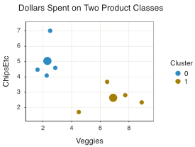
The cluster analysis provides statistics that formalize these relationships. Such numerical information defines how to compute the middle of each group, the cluster center, as well as the distance of each point from each middle.
12.2 Distance Between Samples
How to measure the distance between two samples? How to define a cluster in term of values on all the variables as specified by these distances? The distance between two samples may be computed multiple ways. The most widely used representation of distance is the straight line that connects the samples.
12.2.1 Two Points
To illustrate, consider only two features to allow plotting the data in two dimensions. Begin with two rows of data (samples) for these two variables. When plotted, represent each the two data values in each row of data as a physical point. Then illustrate the literal physical distance between the two points.
Consider two samples (rows of data) from Figure 12.2, each provided by one of two customers. Refer to the following small data table with features Veggies and ChipsEtc.
| Veggies | ChipsEtc | |
|---|---|---|
| Customer A | 7.74 | 2.81 |
| Customer B | 6.48 | 3.68 |
How to plot the data values on the two features for the two customers?
Vector: A variable with multiple values such as a set of coordinates.
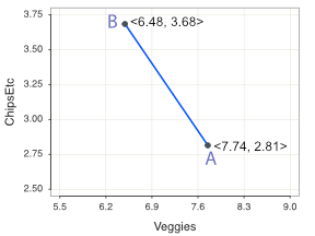
The values of variables Veggies and ChipsEtc for each customer together define a vector. In geometric terms, the vector defines the coordinates of the corresponding plotted point. Here, define the data vector each for Customer A and Customer B. \[A = <7.74, 2.81> \mathrm{and} \; B = <6.48, 3.68>\]
Plotting the data vector for each customer and the line segment that connects them creates the two-dimensional visualization in Figure 12.3.
Now that we have the points, calculate the distance between them.
12.2.2 Euclidean Distance
Define the distance between Points A and B consistent with our intuition: The straight line that connects the two points. The definition of this straight-line distance traces back well more than two millennia.
Euclidean distance: Straight-line distance between two points.
Euclid is the Ancient Greek mathematician from about 300 BC, considered the founder of modern geometry. Of the many ways to assess distance, Euclidean distance is the usual default, and the basis for Euclid’s geometry.
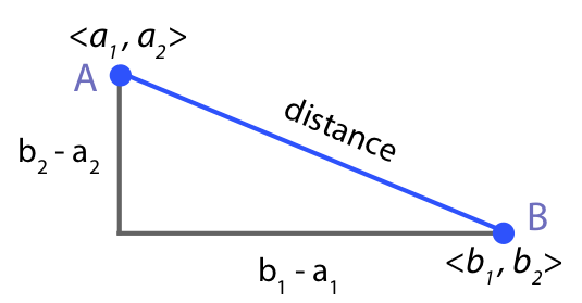
To compute Euclidean distance, we rely upon another Ancient Greek even further back in time, Pythagoras, renowned mathematician and philosopher who wrote around 480 BC. Figure 12.4 shows this straight-line distance between Points A and B as a blue line, the hypotenuse (long side) of the corresponding right triangle, a triangle with a 90 degree angle.
Pythagorean theorem: The length of the hypotenuse of a right triangle (with a 90 degree angle) is the square root of the sum of the squared differences of the length of the other two sides.
Given the differences for each feature across the two points, apply his Pythagorean theorem to calculate Euclidean distance as the length of the corresponding hypotenuse. To compute the distance between the two plotted points for Customers A and B, begin with the calculation of the distance between their corresponding vectors, the data values for each feature, Veggies and then ChipsEtc. Figure 12.4 illustrates these two differences.
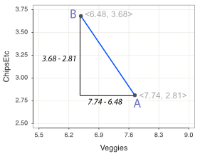
Apply the Pythagorean theorem to calculate the distance between Points A and B in Figure Figure 12.4) as the hypotenuse (long-side) of a right triangle.
\[\mathrm{distance}(A,B) = \sqrt{(7.74-6.48)^2 + (3.68-2.81)^2} = 5.47\]
To calculate Euclidean distance, begin with the length of each of the sides of the triangle about the right angle, square each length, sum, and then take the square root.
12.2.3 Distance Generally Stated
The concept of Euclidean distance as presented in two dimensions generalizes to any specified \(p\) number of dimensions, one dimension for each feature variable. First, consider the general presentation for the distance between two points with two features, generically named \(F_1\) and \(F_2\). Name the rows with generic symbols A and B. Label the corresponding data values as \(a_1\), etc, as shown in the following table.
| F1 | F2 | |
|---|---|---|
| Sample A | a1 | a2 |
| Sample B | b1 | b2 |
The resulting coordinate system, here describing a 2-dimensional plane, provides a visualization of the data values, one point per sample.
Feature space: Each feature corresponds to a dimension (axis) in the coordinate system, and each sample (instance, example) corresponds to a point with data values as its coordinates.
Specify the dimensions with subscripts. In the feature space, the first dimension corresponds to the first feature, so \(a_1\) and \(b_1\) are the scores on the first feature, such as Veggies, for the A and B samples.1
1 A familiar reference to a coordinate system names the horizontal axis \(x\) and the vertical axis \(y\), then specifies the coordinates of a point with subscripts that refer to the corresponding sample. For example, with this notation \(x_1\) specifies the score of the first sample on the variable plotted on the \(x\)-axis. Here use an alternative representation that flips this perspective.
Represent the data values of the two features for two different samples (instances, examples), referenced here as vectors A and B.
\[A=<a_1, a_2> \mathrm{and} \; B=<b_1, b_2>\]
The feature space (also called a vector space) directly represents the values in the data table.
To calculate the Euclidean distance between the points, apply the Pythagorean theorem to as many dimensions (features) as relevant. To illustrate, begin with just two features, as in Figure 12.5. The Pythagorean theorem provides the straight-line distance between the points as the square root of the sum of the squares of the lengths of the two opposite sides. The length of the horizontal side is \(b_1-a_1\), and the length of the vertical side is \(b_2-a_2\).
\[\mathrm{Euclidean \; distance}(A,B) \; \mathrm{across \; two \; features} = \sqrt{(b_1 -a_1)^2 + (b_2 -a_2)^2}\]
In general, there can be, and usually are, more than two features. The Pythagorean theorem for the computation of distance generalizes to as many dimensions as features. Three features imply \(p=3\) measurements for Customer A, so represent the point in a 3-dimensional space with coordinates \(<a_1, a_2, a_3>\). Generalizing further, represent the data values of Row A for \(p\)-features in a \(p\)-dimensional space as vector \(<a_1, a_2, ..., a_p>\).
To calculate the Euclidean distance, apply the Pythagorean theorem feature-by-feature for the two samples (instances, objects, people). Begin with the squared difference of the first feature \((b_1-a_1)^2\). Then, for Rows A and B, continue summing through the sum of squared differences through the \(p^{th}\) feature, \((b_p-a_p)^2\), followed by the square root.
Euclidean distance as the application of the Pythagorean Theorem from Point A to Point B across \(p\) features: \[\sqrt{(b_1 -a_1)^2 + (b_2 -a_2)^2 \; + ... + \; (b_p -a_p)^2} \; = \; \sqrt{\sum\limits_{i=1}^p (b_i -a_i)^2}\]
The generality of this expression provides for computing the distance between any two data vectors, or points geometrically, for any given number of features. Of course, with more than two or perhaps three features, we cannot provide a geometric representation. The underlying definition of distance, however, remains the same.
12.3 \(K\)-means Cluster Analysis
The \(k\)-means solution algorithm for the clusters requires to first specify the number of clusters, \(k\), for that specific analysis.
Obtain \(k\) clusters such that samples within a cluster have similar values on the underlying feature variables X, and dissimilar values on those variables with samples in other clusters.
The \(k\)-means procedure identifies each cluster by the average of each feature across all its constituent samples.
Centroid: Center of a cluster, with coordinates computed as the mean of the corresponding feature values of each sample in the cluster for each feature.
12.3.1 Solution Algorithm
The computational process underlying \(k\)-means cluster analysis is surprisingly straightforward, especially when compared to the mathematical complexity of most machine learning solution algorithms.
Step 0: To begin, choose a random position for the center of each cluster. The initial clusters may be chosen with the constraint that their centers are relatively distant from each other (the default sklearn setting), but otherwise randomly chosen, shown in Figure 12.6.

Step 1. Centroid Distance: Calculate the distance between each sample and each cluster centroid.
Step 2. Cluster Assignment: Assign each sample to the cluster for which the centroid is the nearest distance. For \(k\)-means cluster analysis, indicate the centroid of Cluster \(j\) as the vector \(m_j\). The cluster centroid, then, becomes another point in the plot.
Figure 12.7 shows this distance between a selected point and both cluster centroids from the final solution. The point is assigned to the cluster with the nearest centroid.
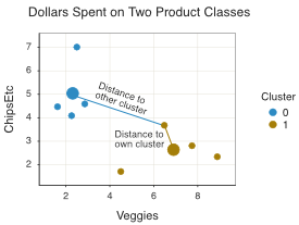
To get these sample-centroid distances, apply the computation of the distance formula of sample A with the computed centroid of the \(j^{th}\) cluster, computed across all \(p\) features.
\[\mathrm{Distance \; of \; Sample \; A \; to \; Cluster \; j: \;}(A,m_j) = \sqrt{\sum\limits_{i=1}^p (a_i-m_j)^2}\]
For each point, perform this computation of sample-cluster distance for each cluster. The algorithm then assigns each point to the cluster with the smallest distance from the point.
Step 3. Centroid Update: Each time a sample is re-assigned to the nearest cluster, the membership of that cluster changes. Shift the cluster centroids around by redefining each cluster. Calculate the new centroid values based on the revised cluster membership. To re-calculate, again take the mean of each feature variable for all the samples in the cluster.
Repeat (iterate) these steps until the process either converges or reaches some maximum parameter value of iterations.
Converged solution: Additional iterations of the three steps for the \(k\)-means solution algorithm leave cluster membership unchanged.
A different choice of initial clusters, however, typically leads to a different cluster solution.
In practice, for a specific number of specified clusters, run several different analyses with different randomly selected starting points for the center of each cluster.
If using Python sklearn, the default setting generates 10 arbitrary initial solutions and then runs a separate cluster analysis for each. The algorithm then chooses the final solution as the initial configuration that yields the best fit (the smallest inertia, explained below). The initial configurations are randomly generated though there is some structure that the initial solutions follow that lead to a more quickly converged solution.
12.3.2 Hyper-Parameter Tuning
As indicated, each \(k\)-means cluster analysis begins from a specified number of clusters to be calculated in a specific analysis. How to know the best number of clusters? One answer is hyper-parameter tuning of the number of clusters based on fit indices. Because the computations are so simple, and thus so fast, usually many different numbers of clusters can be tested.
12.4 Evaluate Cluster Fit
How to evaluate the fit of a cluster solution? A good fitting solution yields clusters in which the samples that belong to that cluster have close distances to the corresponding centroid, and are relatively far from competing centroids. Consider the following two criteria.
Cohesion: Distance of a sample to its own cluster.
Separation: Distance of a sample to other clusters.
A good fitting cluster solution has high cohesion, relatively small distances among its samples, and high separation, relatively large distances to points in other clusters.
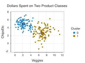
To illustrate, consider a more realistic data of the Veggie and ChipsEtc data, with almost 200 rows of data. Accordingly, the corresponding visualization in Figure 12.8 has almost 200 points. Most of the points, that is, customers, define two distinct clusters. Many points, however, straddle the blue/green cluster boundaries, perhaps defining a smaller third cluster of shoppers who are comfortable with both chips and veggies.
A distinction between the clusters also becomes apparent. Those people who spend more money on fresh vegetables are more scattered than those who focus on chips etc. Some shoppers who spend much on veggies also spend much on chips. Said another way, the grouping of the brown points in Figure 12.8 are more dispersed about their middle than the corresponding grouping of blue points.
12.4.1 Inertia
As we reviewed in in the section on linear regression, one statistical evaluation of fit for a quantitative variable follows from the sum of squared errors, SSE. The errors are the discrepancies between the true value of the target variable and what the model calculates to be true. For \(k\)-means cluster analysis, once the analysis identifies a cluster, even from an arbitrary starting solution, the reference for comparison is the corresponding cluster centroid of which the sample is a member.
The relevant question regards the distance of a sample from the centroid of the cluster to which it has been assigned, the within-cluster distance.
Error: Distance of a point from the centroid of the cluster to which it has been assigned.
As the basis of fit, compute the familiar sum of the squared errors across all samples.
The algorithm assigns each sample to the cluster with which it is the closest. When all samples are assigned to a cluster, evaluate cluster cohesiveness.
Inertia: Total within-cluster variation, the sum of the individual within-cluster variations for all samples.
The \(k\)-means cluster solution algorithm continually re-assigns each sample to its nearest cluster, then re-calculates each cluster centroid. The result reduces inertia on each iteration (or at worst does not increase inertia). When the solution converges, the clusters have the minimal inertia for the given number of clusters, relative to the initial, seeded cluster values.
Hyper-parameter tuning evaluates the fit of the cluster solution across a range of a specified number of clusters. Each individual cluster analysis begins with an analyst specified \(k\) for the number of clusters. Evaluate the optimal number of clusters for the data by systematically varying the value of \(k\), in this context a hyper-parameter.
The cluster inertia always decreases as the number of clusters increases. At first, for a small number of clusters, an increase of one more cluster, such as two, to the next largest number, 3, generally has a dramatic impact on the decrease in cluster inertia. At some point in the tuning, the increase of an additional cluster has less of an impact, such as from 20 clusters to 21.
Elbow method: Estimate the optimal number of clusters \(k\) for a given data set at the point in which the decrease in cluster inertia is relatively small following the addition of an additional cluster.
The elbow method identifies the value of \(k\) where the decrease in the within-cluster SSE begins to decelerate, best revealed by a visualization. The point at which there is relatively less gain for an increase in the number of clusters is the elbow method criteria for setting the optimal number of clusters. Figure 12.9 illustrates the result of hyper-parameter tuning of the number of clusters.
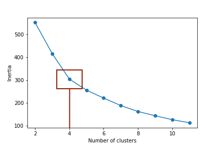
The drop-off becomes smaller after four clusters, suggesting that a four-cluster solution may be more appropriate than the initially proposed two-cluster solution.
12.4.2 Silhouette
Another fit index simultaneously accounts for both cluster cohesion and separation.
Silhouette: Similarity of a sample to its assigned cluster compared to its separation from other clusters.
Compute the silhouette coefficient for each row of data (instance, object, observation, sample). The silhouette coefficient ranges from −1 to +1. The desirable high silhouette value indicates both high similarity and high separation. A value close to 0 indicates that the object is close to a boundary between two clusters. A negative value indicates that the object may be assigned to the wrong cluster.
For each sample (instance, object, point) the silhouette coefficient compares two quantities as a ratio. For a given point, the comparison is between distances to other points in its own cluster to distances of other points to the nearest other cluster. The value, \(a\), is the mean intra-cluster distance, the mean distance of the sample to the other samples within a cluster. The value, \(b\), is the mean nearest-cluster distance, the mean distance between a sample and the samples of the neighbor cluster of which it is not a member.
Silhouette coefficient for a sample: ; \(\dfrac{b - a}{max(a, b)}\)
Because the distance of the point to points in other clusters should be larger than the distance to points in its own cluster, \(b-a\) should be positive, \(b-a>0\).
What is the purpose of the denominator? If \(b\) is positive, then \(b>a\), so divide the numerator by \(b\). The better the fit, the smaller is \(a\) as then the closer the points within each cluster lie to their cluster centroid. When \(b>a\), the silhouette coefficient approaches 1 as \(a\) approaches 0. By dividing by \(b\), or \(a\) if \(a\) is larger, the silhouette coefficient becomes normed, with values that vary from \(-1\) to \(1\) regardless of the specific data analyzed.
To derive a silhouette coefficient for the entire cluster, average each sample silhouette coefficient for all the samples in the cluster. This average silhouette coefficient generally follows a downward sloping pattern, but, unlike cluster inertia, not necessarily. As Figure 12.10 shows, for the cluster analysis of food purchases with almost 200 samples, the coefficient can decrease for each additional cluster, then increase (from 3 to 4 and 7 to 8 clusters), then continue to decrease.
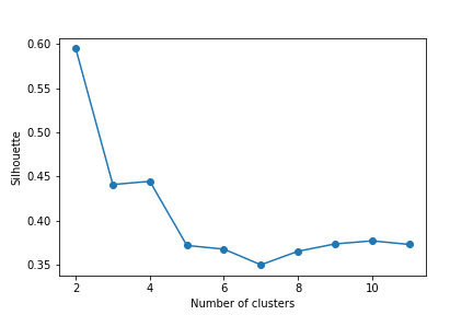
The average silhouette coefficient drops much from a two-cluster solution to the three-cluster solution, but then increases only slightly to four clusters. Adding more clusters typically lowers the coefficient, though not necessarily for each iteration. So the drop from two to three clusters is not surprising. Clearly from this analysis, a solution with 2, 3, or 4 clusters may be the best.
For a specific solution, examine the individual silhouette coefficients across the samples, the rows of data, such as with a histogram. Figure 12.11 illustrates the histogram for the two-cluster solution.
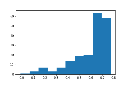
The good news for this interpretation is that most of the silhouette coefficients are above 0.4, and many above 0.6.
12.4.3 Optimal Number of Clusters
Evaluate the fit of each solution with inertia and the silhouette value simultaneously.
Fit strategy: Choose a cluster solution that provides enough clusters to lower inertia, yet maintains a relatively high silhouette coefficient.
The choice of the number of clusters is ultimately subjective, but not without guidance. Examining the changes in inertia and average silhouette systematically across a range of values for the number of clusters provides a statistical basis for the choice. From the corresponding hyper-parameter tuning that displayed these fit indices across a range of number of clusters, consider the four-cluster solution in Figure 12.12.

The statistical analysis of fit suggests that two clusters do not well differentiate among the points, corresponding to the customers. The problem is that with the two-cluster solution, the points more or less continuously vary across the clusters. It is true that many customers clearly go big on veggies and not on chips and related (blue, #1), and other customers do the reverse pattern (red, #0). Many customers, however, do a moderate amount of veggies and almost as many chips and things as do the heavy chip customers, one new cluster (purple, #3). Further many customers do a lot of both types of food purchases (green, #4), another new cluster.
Perhaps the four-cluster solution provides more information. Ultimately, the best choice is the most meaningful choice in terms of, in this case, understanding purchasing decisions. For example, how does the pattern of purchases impact a targeted marketing campaign? Or, depending on the relative margins for chips etc. compared to veggies, where to locate a new store depending on the purchase patterns of those who live nearby?
By better differentiating among types of customers, the four-cluster solution is likely more worthwhile. For example, the customers that remain in the original two clusters are now each more representative of the underlying archetype of a veggie or chip type customer than in the previous two-cluster solution.
Unfortunately, there was not enough data to effectively split the data into training/testing sets. Ideally, the cluster solution would be developed for the training data, then the inertia and silhouette fit indices computed for the cluster centroids on new, testing data.