❝ Descriptive statistics can be like online dating profiles: technically accurate and yet pretty darn misleading. ❞
3.1 Regression Review
We use regression analysis to build a prediction equation. The analysis estimates the values of a specified linear model, which means the computer procedure estimates a y-intercept and a slope coefficient or weight for each X variable in the model, computing the weighted sum. As seen in the section on multiple regression, in practice there are usually several or more predictor variables. Ten examples of different sets of predictor variables, each set predicting a different target or response variable were provided in the introductory section called Prediction Equation. From the data values for each set of variables, the corresponding model is estimated.
As discussed, the two purposes of regression analysis follow from the relationships of a set of features or predictor variables \(X\) to a target or response variable \(y\).
- \(\hat y\): Predict (forecast) unknown values of \(y\) from given values of variables \(X\).
- \(b\): Understand how changes in the values of one or more \(X\) variables relate to changes in the values of \(y\).
In some analyses, concern may focus on only one of these goals. In other analyses, there is interest in both. Here, focus on the second purpose, estimating the extent of the relationships. To begin, consider just a single predictor variable, \(x\). The presented example continues from the previous section, estimating a person’s weight from their height. Estimation in terms of minimizing a function of the residuals was also considered in the previous section. Here the focus shifts from using the obtained model to describe the given data to generalizing the results beyond the sample to the population as a whole, always the concern of applied analysis.
3.2 Sample vs. Population
Regression analysis estimates the slope of the regression line, the estimate indicated by \(b_1\). The slope informs us as to how much \(y\) changes, on average, as \(x\) increases by a single unit. The sample slope coefficient, \(b_1\), informs us as to the subsequent change in \(y\) only for that sample of data from which the model was estimated, the training data.
3.2.1 Population Values
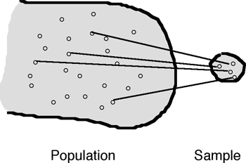
All statistical computations, such as for a slope coefficient, \(b_1\), are necessarily based on a sample of data values from a larger population, not the population itself.
Sample from the larger population to obtain data for analysis.
Figure 3.1 illustrates.

The population may consist of a usually large number of fixed elements in a given location at a given time, such as all registered voters in the USA. More broadly, the population consists of the outcomes of an ongoing process, in which case the population and its associated values are hypothetical, having not yet occurred.` The population contains the desired information, which can only be estimated – guessed at – from the corresponding sample values.
Examples of population values include the population mean for a given variable and the population slope coefficient for a given regression analysis. A population value is an abstraction, considered real, but not observed, its value unknown, but the desired value.
Statistical notation indicates a statistic calculated from the sample data, such as \(b\), with Roman letters. The corresponding Greek letter denotes the corresponding population value, such as the Greek letter beta.
Express the desired population version of the model we estimate from the data with \(\beta\)’s instead of b’s. \[\hat y = \beta_0 + \beta_1(x)\]
To review a specific example of the analysis of such a model, return to the example of predicting a male customer’s weight (\(y\)) from his height (\(x\)).
We do not observe the entire population, so the desired true values, the population values, are not available for analysis. Our knowledge of a population value of interest, such as the slope coefficient, \(\beta_1\) or the \(y\)-intercept, \(\beta_0\), is limited to information we derive from a (presumably random) sample from the population. And that is the crux of the problem.
Flip a fair coin 10 times and you may get four heads, for 0.4 proportion. Flip the same coin another 10 times and you may get six heads, for 0.6 proportion. Neither value is the correct population proportion of 0.5. The true population proportion is best defined as the long-run average, the proportion of heads obtained over an indefinitely large number of coin flips.
Examples of such statistics computed from any one sample are the sample mean and the sample slope coefficient from an estimated regression model.
Consequence of sampling error: For each new sample of \(X\) and \(y\) values, different values of the slope coefficient \(b_1\) and \(y\)-intercept, \(b_0\) would be obtained.
As illustrated in Figure 3.2, each distinct sample yields a different regression line. Conceptually, the sample regression line randomly fluctuates from random sample to random sample about the true, population regression line.
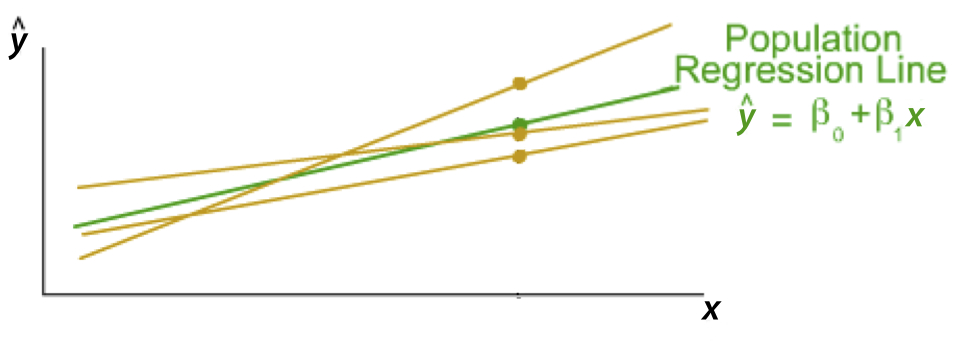
In practice, the analysis consists of only one sample, with only one regression line estimated. Every statistic computed from a sample of data, such as a mean or slope coefficient, only estimates the corresponding population value. More bluntly, every estimate of \(\beta_1\) is wrong. The sample slope coefficient is not the corresponding population slope coefficient, \(b_1 \ne \beta_1\).
To properly interpret a model, interpret the estimated population values of the coefficients.
We cannot directly observe the population values that we wish to know. What to do? We generalize from the arbitrary sample value to the true population value that characterizes the population as a whole.
The obfuscation that results from the ever-present sampling error motivates the development and application of inferential statistics. A sample estimate only describes a sample of data. Inferential analysis generalizes that estimate to the population with an interval at a specified probability. For a given population value, some samples are more likely than others.
Report every computed statistic that describes a particular sample with its corresponding inferential analysis.
Even if we correctly specified the model we do not know the true values of the regression coefficients: Population y-intercept, \(\beta_0\) and slope, \(\beta_1\). In the future we will never again observe the particular sample from which we estimated the model.
We calculate statistics that describe the sample but infer the corresponding characteristics of the population from which the sample was derived.
We care about the population from where the sample was obtained, not a description of the particular sample we did obtain. We use statistical inference to estimate the values of the estimated model such as the slope coefficient.
3.2.2 Standard Error
How to estimate the value of the unknown population value, such as \(\beta_1\). We have a single estimate, \(b_1\), but that estimate is wrong, \(b_1 \ne \beta_1\). How wrong? To answer that question, rely upon the fact that every sample produces a different estimated value of the statistic of interest.
Because sample results vary from sample to sample, over many different samples a statistic such as the slope coefficient becomes a variable. Of course, we only have one sample, so we only compute one value of a statistic from this sample. However, using formulas from the mathematicians we can estimate what would happen if we observed multiple samples. These formulas provide the answers from the information in only a single sample. These formulas are then programmed into the computer code for doing a data analysis, such as linear regression.
How much does \(b_1\) vary from sample to sample, all samples of the same size from the same population? We cannot know \(\beta_1\) directly, but if we have many values of \(b_1\) from many samples and know their variation, we get closer to knowing the value of \(\beta_1\). The distribution of the sample values of the statistic over these hypothetical multiple samples is called it’s sampling distribution, which is normal according to the central limit theorem.
What statistic indicates variability? That statistic is the standard deviation. Understanding statistical concepts that we apply to data analysis is impossible without understanding the definition and meaning of the standard deviation.
If the standard deviation of a statistic over (usually hypothetical) repeated sampling is low indicating little variability, then the estimate from any one sample is likely close to the unknown population value.
If the value of the statistic does not vary much over many samples, than any one value of that statistic from any one sample is likely to be close to the true population value.
If one sample of a specific size of paired values \(x\) and \(y\) yields a value of \(b_1=2.41\), another sample yields \(b_1=2.40\), and another sample yields \(b_1=2.42\), we would feel reasonably confident that the true value \(\beta_1\) is right around 2.41, and not, for example, 300 or even 3. The three estimated values of \(b_1\) over repeated samples vary only a little, so they have a small standard deviation, here only 0.01. Any one sample value of these three values is likely close to the true value, \(\beta_1\).
In contrast, if three equivalent samples of paired \(x\) and \(y\) values yielded \(b_1=2.41\), \(b_1=11.62\), and \(b_1=6.15\), we would have little confidence that any one \(b_1\) is close to the true value \(\beta_1\). The standard deviation of these three values is 5.63, much larger than the value of 0.01 in the previous example.
A standard error is a standard deviation. We usually reserve the term standard deviation, however, to describe the variability of the data in a single sample. The standard deviation of a statistic over (usually hypothetical) repeated samples is named standard error. The size of the standard error indicates the extent of the error in estimating the underlying true value. A large standard error indicates little confidence that any one sample statistic is close to the underlying true, population value.
Knowing the standard error of the distribution of the statistic and knowing that the distribution is normal, gives us information we need to calculate the corresponding probabilities. These values of a statistic over multiple samples form a distribution. Describe any distribution, in part, by its mean and standard deviation, called the standard error if applied to a distribution of a statistic.
The key conceptual basis of inferential analysis of a statistic is its standard error. According to the central limit theorem, except in very small samples from non-normal populations, the distribution of a statistic is at least approximately normal. In that case, apply normal curve probability to evaluate the extent of the error: The two standard error (deviations) about the middle accounts for about 95% of the values. The exact 95% cutoff is 1.96 standard deviations, and, as shown in Figure 3.3, 95.5% for two standard deviations on either side of the mean.

The standard error with this 95% rule, applied to the hypothetical distribution of a statistic over repeated samples, becomes the “yardstick” by how we do statistical inference. Note that this hypothetical distribution, usually normal (by the central limit theorem), is not the distribution of the data, which may or may not be normal. We have one distribution of the data itself, and a second, usually hypothetical distribution, of a statistic we would calculate from many samples of data.
3.3 Two Forms of Inference
Based on the standard error, two forms of (classical) inferential analysis infer the value of an unknown population value. These inferential analyses apply to any statistic that estimates a population value, such as the slope \(\beta_1\) from the estimate \(b_1\). The two forms of inference are the hypothesis test and the confidence interval, both of which provide complimentary and necessarily consistent information.
3.3.1 Hypothesis Test
The hypothesis test focuses on a specific population value (or range of values) of interest for purposes of the test. The so-called “hypothesis” is a somewhat misleading term because it is not necessarily a hypothesis as a statement that the researcher endorses and seeks to support. The so-called hypothesis is a single value (or range of values) that the researcher tests, often with the intention to disconfirm that value.
The hypothesis test is all about the analysis of what is expected from the value that is tested. If you hypothesize no relationship between \(x\) and \(y\), then you hypothesize that \(\beta_1=0\). IF that presumed value of 0 is true, then what value do you expect for the corresponding sample estimate, \(b_1\)? The answer is that you expect a value close to 0, but not exactly equal to 0. The value of \(b_1\) close to 0 if \(\beta_1=0\) is exactly the same situation if you flip a coin 100 times that you hypothesize to be fair. If the coin is fair, you do not generally expect to get exactly 50 heads but you do expect a value close to 50. If the number of Heads is 75, then the probability of this result is very small, so the null hypothesis of a fair coin is likely false.
Where does this hypothesized value come from? The hypothesized value arises from the analyst, from you. Choose the value of primary interest. For assessing the slope coefficient, the value of interest usually indicates no relationship between \(x\) and \(y\). In the case of no relationship, a unit increase in \(x\) does not lead to any systematic change in the corresponding value of \(y\) up or down. Increase the value of \(x\) by one unit and the value of \(y\) in this circumstance is as likely to increase as decrease.
A hypothesis test of what is called the null hypothesis, applied to the population slope coefficient, \(\beta_1\), assumes no relationship between \(x\) and \(y\). Denote the null hypothesis with \(H_0\).
The null hypothesis specifies the value to evaluate. Identify the alternative to the null as \(H_1\) or \(H_A\). The alternative is whatever the null is not, here \(H_1: \beta_1 \ne 0\), which specifies that \(x\) and \(y\) are related in either a positive or negative direction. According to tradition, the alternative to the null hypothesis is misleadingly called the alternative hypothesis, but it is not directly tested. The test is of the null hypothesis.
For purposes of the hypothesis test assume the null hypothesis of \(\beta_1=0\) is true,
Regardless if the analyst wishes to disprove or not disprove the null hypothesis, assume, for purposes of the test, that they are not related. Then evaluate how close the sample value of \(b_1\) is to zero. Does the sample value of \(b_1\) meet the expectation consistent with the null hypothesis, that is, a value close to 0?
The focus of the inferential test for the population slope coefficient \(\beta_1\) is the null value of 0.
- If \(\beta_1\) < 0, x negatively relates to y
- If \(\beta_1\) = 0, no relationship of x and y
- If \(\beta_1\) > 0, x positively relates to y
Even if there is no relationship, \(\beta_1=0\), the sample slope coefficient will not equal zero, \(b_1 \ne 0\). If, however, \(\beta_1=0\), then \(b_1\) should be close to 0. IF, as assumed for purposes of the test, the null hypothesis of a zero population slope coefficient is true, THEN the sample slope coefficient over repeated samples would randomly vary about 0.
If \(b_1\) is close to 0, then the result is consistent, but does not prove, the null hypothesis of no relation, \(\beta_1=0\). Many other values of \(\beta_1\) could produce a sample value \(b_1\) close to 0. On the contrary, if \(b_1\) is far from 0, then very likely the null hypothesis is false. A sample value \(b_1\) far from zero renders the population value of \(\beta_1=0\) implausible.
The hypothesis test evaluates the distance of the sample result, \(b_1\), from the null hypothesized value of 0. The sample result. Is \(b_1\) is so far from 0 that the value of 0 for a population result is rendered implausible? IF the null hypothesis of no relation is true, is our sample value \(b_1\) a weird, improbably result? Or, is it consistent with the null hypothesis? The situation is exactly the same as flipping a coin 100 times. You get 53 heads and conclude the coin is likely, though not necessarily, fair. You get 83 heads and you conclude that the coin is likely not fair.
Consider the hypothesized value plausible if the sample value lies within the 95% range of variation of the statistic about the hypothesized value. If the sample value lies outside this range, in the 5% probability range, then consider the hypothesized value implausible.
Applying normal curve probabilities, the 95% range of variation of the statistic follows from the normal curve cutoff of 1.96 standard errors on either side of the true value, here assumed to be 0. In practice, this result is theoretical because we do not know the true standard error, but must estimate. That leads to the family of \(t\)-distributions, with probabilities computed from the estimated, not the actual, standard error. To compute a \(t\)-statistic requires not only a sample mean, but also a sample standard deviation.
The result of using a \(t\)-distribution with this additional source of variability is a little wider cutoff than 1.96 to get the 95% range of variation of the statistic, shown in Figure 3.4. The distribution is of the hypothetical sample slope coefficient \(b_1\) estimated over many, many different samples, mathematically derived. Values of \(b_1\) less than about two standard errors from 0 are considered plausible given the assumption of the population value of \(\beta_1=0\). From this assumption of the null, 0 is the center of the presumed distribution.
Because a 95% range of variation, \(\alpha = 0.05\), leaves 2.5% in each tail, indicate the mathematically determined \(t\)-cutoff value as \(t_{.025}\). This value is always larger than the corresponding \(z\)-cutoff=1.96, with a value around 2 except for very small sample sizes. The value is larger for small sample sizes and closer to 1.96 for large sample sizes.
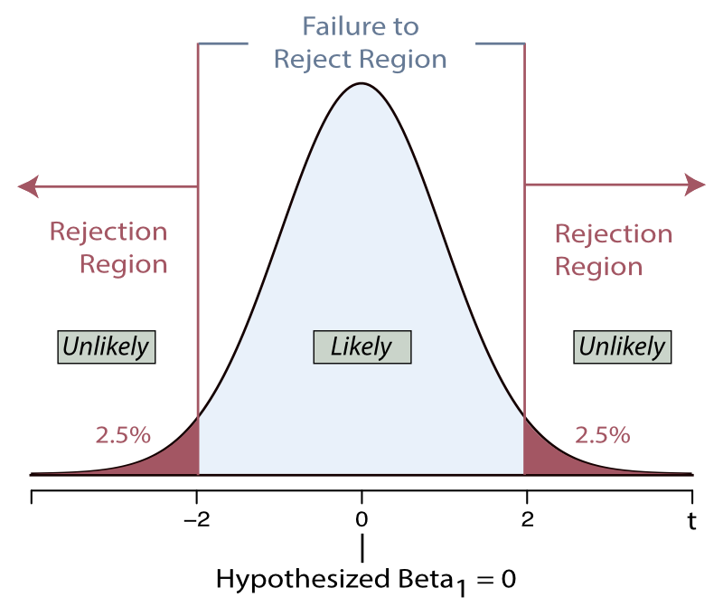
Figure 3.4 does not show any results of a data analysis. Figure 3.4 illustrates a purely mathematical result based on a hypothetical result, a statistic computed over multiple samples with an assumed center of 0 for purposes of the test.
Now compare the theoretical distribution to a data outcome. The sample \(b_1\) is always different than zero. The question of interest is if the value of \(b_1\) is so far from zero that zero becomes implausible? Assess distance in terms of the standard error, which pinpoints location along a normal curve, or a related \(t\)-curve
A \(t\)-value larger than the \(t\)-cutoff of about 2 or smaller than -2, indicates an improbable event IF the null hypothesis is true. Corresponding to how far \(b_1\) is from zero, we can compute the probability of this obtained value, again, assuming the null hypothesis.
The \(t\)-value shows how many standard errors is the sample result from the null value, here 0. The \(p\)-value shows how compatible the data are with your underlying assumption of the null hypothesis. The \(p\)-value is a probability, a value between 0 and 1. What is the probability of the sample result as far or farther from the null value, assuming the null value is true. Either one of these statistics implies the other, so they provide equivalent information. A large distance from the assumed value, the \(t\)-value, implies a small probability that such a result occurred, the \(p\)-value, and vice versa.
Any sample value within the 95% range of the statistic’s variability over repeated sampling is considered plausible, illustrated with an example in Figure 3.5. The \(t\)-value of 1.05 is small, so the equivalent \(p\)-value of 0.30 is large.
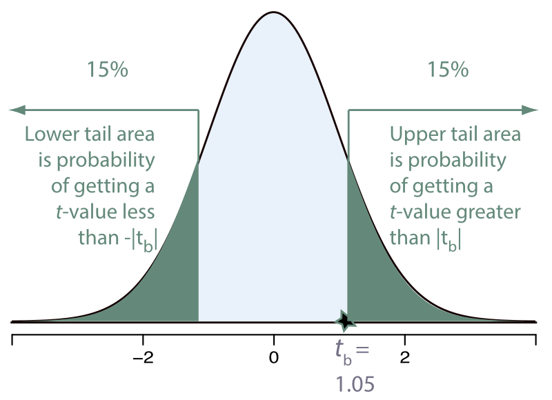
This 95% range of plausibility corresponds to \(\alpha=0.05\) or 5% or less probability of an event occurring defined as weird or implausible. Any value outside of 95% range is considered implausible if the null hypothesis true.
If \(p\)-value \(> \alpha=.05\), conclude no difference detected from 0, that is, a relationship was not detected.
Note that the relationship may exist, just that it was not detected in this analysis.
Alternatively, given the assumption of the null hypothesis, Figure 3.6 illustrates an improbable event defined according to the cutoff defined as \(\alpha=0.05\).
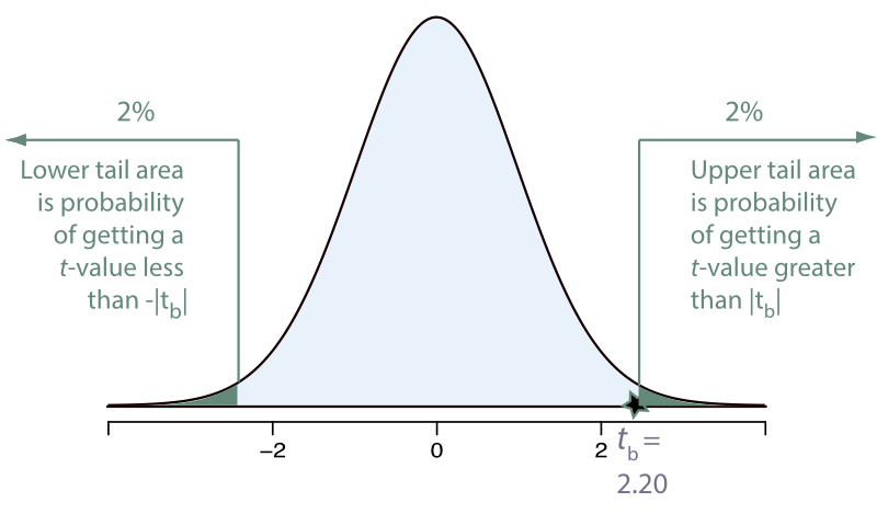
The large \(t\)-value and equivalent small \(p\)-value both describe the same data, and provide the same information. The \(t\)-value shows that the sample value of the statistic, here \(b_1\), is far from the hypothesized population value in terms of standard errors. The corresponding \(p\)-value provides the corresponding small probability assuming 0 is the correct population mean, here considering both directions. The \(p\)-value is below the proposed definition of implausible, less than \(\alpha=0.05\).
If \(p\)-value \(< \alpha=.05\), conclude a difference detected from 0, then state the direction of the relation, positive or negative.
Note that the hypothesis test begins with an assumption, so all conclusions start with this assumption. If the null is false, then expect a sample value, \(b_1\), to be “far” from zero, specifically more than two standard errors. If the null is rejected, then 0 is probably not the true value of \(\beta_1\). Instead, it is greater than or less than 0, which implies a relationship between \(x\) and \(y\). As the value of \(x\) increases, the value of \(y\) tends to either systematically increase or decrease.
3.3.2 Confidence Interval
If the null hypothesis of a zero slope-coefficient is rejected, the natural follow-up question to ask: What is the size of this slope coefficient? Use the confidence interval to estimate the size of the relationship. Interpret this confidence interval in terms of the meaning of the slope coefficient.
Note that the preceding statement is a definition, not an interpretation of the results delivered to management.
Usually choose the 95% range of variation to define the 95% confidence interval, which implies that 95% of the sample values of \(b_1\) across repeated samples would be within about two standard errors of the true value, \(\beta_1\), whatever its value.
Given the range that defines 95% of the sample statistics about the true population value, place that range over the obtained value of the sample statistic to likely contain the true population value.
Figure 3.7 illustrates an example of when the true population value, here \(\beta_1\), lies within the confidence interval. The true population value is the center of the distribution of the corresponding statistic, under the assumption of the null hypothesis, over repeated samples. Because the sample mean and sample standard deviation vary for each sample, the computed confidence interval is also a different interval for each samples. On average, however, over many samples each of the same size, 95% of the corresponding confidence intervals contain \(\beta\).

View a video [4:49] that develops Figure 3.7 step-by-step.
Unlike the hypothesis test, construction of the confidence interval does not involve any pre-specified value. Instead, construct the confidence interval only from sample information.
Construct the confidence interval as the range of plausible values spans approximately two standard errors on either side of the sample value.
The elegance of the logic displayed in Figure 3.7 is that to construct the confidence interval, the true value of \(\beta_1\) need not be known, and, in practice, is not known. Estimating its value is the entire point of this exercise.
Ultimately our results concern the population. All conclusions regarding the inferential analyses are in terms of the population. The sample slope coefficient \(b_i\) describes this relationship for the sample. Instead, we want this analysis for the unknown population value \(\beta_1\). We do not know its value, but with the confidence interval we have a probability (such as 95%) that the value lies within the specified range. The downside is that risk cannot be avoided: In practice we only observe a single sample, so we do not know if that sample is one of those occasional samples that does not contain \(\beta\). The confidence interval for 5% of the samples fails to contain the unknown population value.
3.3.3 Consistency
If constructed with the same range of variation, both the hypothesis test and confidence interval, such as 95%, necessarily are consistent with each other. A rejected hypothesized value such as 0 will not lie in the confidence interval. Both the hypothesis test and the confidence interval in this situation indicate that 0 is implausible in this situation.
On the contrary, a non-rejected hypothesized value such as 0 indicates that 0 is plausible. By definition, the confidence interval contains the range of plausible values of the true, population value. So if 0 is plausible from the hypothesis test, it will also lie within the corresponding confidence interval.
3.4 Example
The ultimate purpose of an analysis communicates results to those who hired you to conduct the study. Follow these three principles when constructing your report.
- Communicate the analysis results in terms of population values.
- Apply each interpretation of the results to the specific variables and numerical results to the analysis being conducted, do not just repeat general definitions.
- Apply the results in terms of the meaning of the underlying parameter, not just a verbal restatement of the statistical result.
3.4.1 Estimated Model
Consider an example based on 169 adult male customers. If an online order is placed with customer’s weight missing from the order, how to predict a customer’s weight from his height?
First read the data.
#d <- Read("http://web.pdx.edu/~gerbing/data/regEg_data.xlsx")
d <- Read("data/regEg_data.xlsx")
[with the read.xlsx() function from Schauberger and Walker's openxlsx package]
Data Types
------------------------------------------------------------
integer: Numeric data values, integers only
------------------------------------------------------------
Variable Missing Unique
Name Type Values Values Values First and last values
------------------------------------------------------------------------------------------
1 Height integer 169 0 16 76 71 67 ... 69 72 69
2 Chest integer 169 0 24 44 41 38 ... 42 44 40
3 Weight integer 169 0 61 230 187 145 ... 160 185 180
------------------------------------------------------------------------------------------With the data available, proceed with the analysis.
☞Identify the response or target variable and the predictor variable(s) or feature(s). Weight is the target or response variable, generically referred to as Y. Height is the feature or predictor variable, generically referred to as X.
Do the regression analysis assuming a linear model, estimating the parameters \(b_0\) and \(b_1\) of the corresponding linear model.
☞Enter the function call, the instruction, to obtain the analysis. reg_brief(Weight ~ Height)
The output for the estimated model appears in Figure 3.8.

The first consideration is the estimated model. The machine learned that \(b_0=-393.788\) and \(b_1 = 8.520\), the values that minimize the sum of the squared errors across all 169 customers. Let w and h represent weight and height, respectively.
☞Write the estimated regression model. \(\hat y_{w} = -393.788 + 8.520(x_{h})\)
3.4.2 Slope Coefficient
In this particular sample, \(b_1=8.520\).
☞Specify and interpret the sample slope coefficient. In this particular sample of 169 adult males, for each additional inch of height, weight, on average, increased just over 8 1/2 lbs.
This description of what happened in this one sample, however, is not our primary interest. Our concern is the value of the slope coefficient for the population as a whole, obtained with the inferential analyses. The focus shifts from what describes the particular sample that we encountered to what is the true population value of the slope coefficient, \(\beta_1\)? Obtain he best generalization of the results to future applications from knowledge of the corresponding population values.
3.4.2.1 Hypothesis Test
The hypothesis test informs as to if the relationship likely exists in the population, and, if detected by rejecting the null value of 0, its direction, + or -.
Begin the process of the hypothesis test with the assumption of the null hypothesis, the hypothesis of no population relationship. Assume the null hypothesis is true for purposes of the test. We do not know if the null hypothesis is true, and we more often than not are willing for it to not be true. But we assume that it is true for purposes of the test. The alternative to the null hypothesis is that there is a relationship between \(x\) and \(y\) in the population.
General Statement of the Null Hypothesis, \(\; H_0: \beta_1=0\)
General Statement of the Alternative to the Null Hypothesis, \(\; H_0: \beta_1 \ne0\)
☞ Specify the null hypothesis and its alternative for the hypothesis test of the slope coefficient.
The null hypothesis states that in the population, as Height increases, Weight does not systematically increase or decrease, no relation: \(H_0: \beta_{Height}=0\).
The alternative to the null states that increases in Height are associated with a change in Weight, on average, positive or negative: \(H_1: \beta_{Height} > 0\) or \(\beta_{Height} < 0\).
The hypothesis test evaluates how close the sample result, here \(b_1\), is to the hypothesized population value, here \(\beta_1\). That evaluation of distance is in terms of the standard error of the sample estimate, here \(s_b\), where the \(b\) refers to the sample slope coefficient. Understanding the concept of standard error is essential to understanding inferential statistics, such as the hypothesis test.
☞ Include and apply the definition of the \(t\)-value with the relevant numbers for this analysis of the specified slope coefficient.
The \(t\)-value is how many standard errors the sample result, \(b_{Height}=8.520\), is from the null hypothesis value of \(\beta=0\). \[t_b = \frac{b_1 - 0}{s_b} = \frac{8.520}{0.983} = 8.665\] The \(t\)-value shows that \(b_{Height}=8.520\) is a very large 8.665 standard errors from 0.
By itself, we do not know if any one \(b_1\) is close or far from 0 in terms of the probability of obtaining such a result. We need to express the distance in the metric of the standard error of \(b_1\), the standard deviation of \(b_1\) over (hypothetical) repeated samples. The standard error of \(b_1\), \(s_b\), indicates how much \(b_1\) varies from sample to sample. This range of variation provides the baseline for evaluating how far any one \(b_1\) is from 0. If 0 is the true value of \(\beta_1\), then 95% of the values of \(b_1\) should lie within about 2 standard errors (deviations) on either side of 0.
☞ Include and apply the definition of the p-value with the relevant numbers for this specific analysis.
IF the null hypothesis of no relationship between Height and Weight is true, then the sample \(b_{Height}\) represents a very unlikely event, with a probability of \(p\)-value \(=0.000\) to three decimal digits.
This \(t\)-value is well, well beyond the approximate value of 2 that defines the 95% range of variation of \(b_1\) over repeated sampling. The \(p\)-value provides the probability of the getting a value of \(b_1=8.520\) that far from 0, about 8 and 2/3 standard errors, if the null hypothesis is correct. IF the null hypothesis of no relationship is true, an extremely unlikely event occurred. Here, p$-value \(\approx 0.000\).
>☞ Specify the basis for the statistical decision for the hypothesis test and the resulting statistical conclusion for alpha=0.05 for this analysis of the specified slope coefficient.
Reject the null hypothesis because the \(p\)-value=0.000 \(< \alpha = 0.05\).
The relationship observed in the sample apparently generalizes to the population as a whole, that is, \(\beta \ne 0\). Of course, after doing the analysis, you would not inform management just that there is a relationship but also the direction of the relationship, positive or negative.
☞ Hypothesis Test: Interpretation, as an executive summary you would report to management.
Weight and height are related. As height increases, weight, on average, also increases.
Use statistical jargon such as “null hypothesis” and “p-value” for statistical reasoning in the above questions, but avoid the jargon for interpreting the results. The interpretation is for the benefit of management. Do not assume that managers are statistical geeks. Managers want results explained in plain English (or whatever). State that \(x\) is related to \(y\), using the actual variable names, not the generic \(x\) and \(y\). State the qualitative nature of the relationship, + or -.
Also, note that there is nothing in the interpretation about the sample slope coefficient, \(b_1\). Nor is there anything about the value of the population slope coefficient in the interpretation, \(\beta_1\). Instead, the hypothesis test simply informs us as to the plausibility of the null hypothesis value of \(\beta_1=0\). The hypothesis test does not inform us regarding the size of the population slope coefficient.
3.4.2.2 Confidence Interval
If the hypothesis test detects a relationship between the two variables of interest, a follow-up question naturally emerges. What is the extent of the relationship as indicated by the slope coefficient? What is our best assessment of how much \(y\) changes for a unit increase in \(x\) for the true, population value of the slope coefficient, \(\beta_j\)? We cannot provide a precise estimate of \(\beta_j\). Instead we provide an interval that likely contains the true value.
☞ Specify the value that the confidence interval estimates.
The confidence interval estimates the value of \(\beta_1\), the population slope coefficient for Height as related linearly to Weight.
To report the extent of the relationship, examine the confidence interval of the slope coefficient, which estimates the true \(\beta_1\).
To calculate the estimated value of the slope coefficient, \(b_1\), and its standard error, \(s_b\), along with basic summary statistics such as the means of the variables,the computer does much work. However, given these initial calculations, deriving the confidence interval requires only a little arithmetic. Begin with the margin of error.
Again, the underlying concept is based on the standard error of the statistic of interest, here \(b_1\). Understanding that concept adds much clarity to understanding the entire analysis. Otherwise the ability to understand the results becomes more an arbitrary memorization of a bunch of symbols instead of a meaningful, logical progression.
☞ Apply the definition of the 95% margin of error for its computation using the relevant numbers of this analysis with 2 approximating the t-cutoff from this analysis of the specified slope coefficient.
The margin of error is about two standard errors. \[\textrm{Margin of Error}: t_{.025}(s_b) = 1.974 (0.983) = 1.94\]
The number “two” is the approximate cutoff for a 95% range of variation for a \(t\)-distribution, an approximation to the normal curve without knowing the true standard error. The confidence interval for 95% range of variation is about two standard errors, the margin of error, on either side of the sample value.
☞ Show the computations of the 95% confidence interval illustrated with the specific numbers from this analysis of the specified slope coefficient.
From the margin of error, obtain the confidence interval.
\[\textrm{Lower Bound: } 8.520 - 1.94 \approx 6.579\] \[\textrm{Upper Bound: } 8.520 + 1.94 \approx 10.461\]
However, reporting the confidence interval is not its interpretation. To communicate its meaning, include the definition of the slope coefficient in its interpretation.
☞ Confidence Interval: Interpretation, as an executive summary you would report to management.
With 95% confidence, for each additional inch of height, weight, on average, for all the people in the population, increases somewhere between 6.58 and 10.46 lbs.
As always with interpretations, management cannot be expected to know, or even care, about some weird thing called a \(\beta\). Drop the jargon. The interpretation of the slope coefficient replaces the jargon with its meaning.
The general template for interpreting the confidence interval of a slope coefficient follows.
| Interpretation | Purpose |
|---|---|
| With 95% confidence, | State the Confidence Level |
| for each additional inch of height, | Increment predictor by one unit |
| weight, on average, | Variable to predict |
| for all the people in the target population, | Generalizability of results |
| increases somewhere between | CI is a range, not a single value |
| 6.58 and 10.46 lbs | CI of population slope coefficient |
Everyone can understand the meaning of an interpretation, mercifully spared the statistical jargon.
3.4.2.3 Consistency
Both forms of statistical inference discussed here generalize a sample result to the population.
- The hypothesis test tells us if a relationship exists, if the population slope coefficient is likely different from zero, from which we can infer the direction, + or -
- The confidence interval estimates the extent of the relationship, a range of plausible values of the population slope coefficient
☞ Demonstrate the consistency of the confidence interval and hypothesis test using the specific numbers for this analysis for both results.
The hypothesis test rejects 0 as a plausible value of \(\beta_{Height}\). The confidence interval indicates the range of plausible values of \(\beta_{Height}\), which spans from 6.58 to 10.46, so the value of 0 lies outside the confidence interval. Both analyses indicate that there is a positive relationship between height and weight. <>
The hypothesis test and the confidence interval, both based on the same 95% range of (usually hypothetical) repeatedly sampled values of \(b_1\), provide complementary but consistent results.
With the confidence interval, there is no particular need for a hypothesis test, which only provides the \(p\)-value as additional information. That test is included here because it is included in all explanations of traditional statistical inference. There is a natural progression of doing the hypothesis test, and then, if not significant, no difference detected, then no particular reason for the confidence interval which will then contain 0 as a plausible value, as well as both contradictory negative and positive values.
3.4.3 Model Fit
A regression analysis yields an estimated model when applied to virtually any set of data. The fact that a model was estimated, however, does not indicate that the model effectively describes the data.
A model that fits the data well has smaller residuals, \(y_i - \hat y_i\), than does a model that poorly fits the data.
As previously defined, two fit statistics summarize the extent of the residuals as they exist for this particular data set. Obtain both descriptive fit indices as transformations of the sum of squared residuals: \(s_e\) and \(R^2\). Report these fit statistics for every regression analysis. Figure 3.10 shows the output from Regression().

☞ Evaluate fit with the standard deviation of residuals.
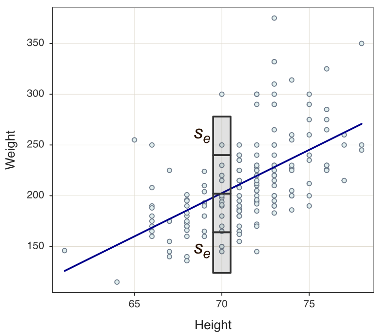
The standard deviation of the residuals, \(s_e\), describes the extent of variation about the regression line, assumed the same for each value of \(x\). In this analysis, \(s_e= 38.039\). This value is fairly large, given that the 95% range of variation about each value of \(x\) on the regression line is 4 times \(s_e\), or over 152 lbs.
The larger the variability about each fitted value on the regression line, the worst the predictive power of the model. And, as shown in the next section on Prediction, prediction in practice will be worse than the \(s_e\). The reason is that sampling error also contributes to prediction on new data, that is, actual prediction.
Figure 3.10 illustrates this range of variation with two units of \(s_e\) about the regression line, with the value of \(x=70\) arbitrarily chosen. Because prediction applies to new data fro which the model was not optimized, the prediction intervals will be even larger.
☞ Evaluate fit with \(R^2\).
The \(R^2\) value of 0.31 indicates that the model is somewhat fitting the data in the sense that the slope of the regression line reduces the sum of the squared residuals compared to the null or flat-line model, though with considerable room for further improvement.
The null model computes each \(\hat y\) as \(m_y\), the sample mean of \(y\), for all values of \(x\). The size of the residuals using height as a predictor of weight reduces the sum of the squared residuals by 31% from the null model. Further, this reduction in the size of the residuals is statistically significant, shown by the test of the null hypothesis that all slope coefficients are zero, with \(p\)-value \(<0.05\) and more, zero to three decimal digits.
How to modify the model to improve fit? One possibility is the functional form. Perhaps a non-linear relationship such as logarithmic or a power function would improve fit. In this example, however, the relationship between height and weight appears at least roughly linear. The best alternative in this situation adds more predictor variables to the model, such as the chest size measurement. This enhanced model is called a multiple regression model.