❝ Prediction is difficult, especially when dealing with the future. ❞
4 Concept
Exponential smoothing is the most widely used of the many available time series forecasting methods. What is “smoothing” and why is it “exponential”? These questions are answered below, but first, a review of basic vocabulary that applies to all predictive model-building methods.
Choose a type of predictive model, such as exponential smoothing, estimate specific details of that model from the data analysis. Evaluate some aspects of its effectiveness by having the model attempt to reconstruct the data. These procedures have been discussed in more detail in linear regression, especially Section~2.4 on Residuals. These same concepts are briefly reviewed here but applied to time series data.
When developing a model with a single predictor variable, we require two columns in our data table: values of the variable from which to forecast and current values for the variable we wish to predict future, unknown values. With time series data, the variable from which we seek to forecast, the predictor variable, is Time. Table 4.1 depicts the general form of the data table.
| Time | y |
|---|---|
| 1 | \(y_1\) |
| 2 | \(y_2\) |
| 3 | \(y_3\) |
| … | … |
| n | \(y_n\) |
In practice, the time values are usually entered not as numbers but as dates, such as 08/18/2024. These dates can represent data collected daily, weekly, monthly, quarterly, or annually. The variable with values to be predicted is generically referred to as \(y\), a variable such as Sales or Production output. Generically, the variable’s specific data value is referred to as \(y_t\), the value of \(y\) at Time \(t\).
Existing data values from which the forecasting model has been estimated.
Submit the data organized as in Table 4.1 to a computer program that can perform the exponential smoothing forecasting analysis. The analysis results in a model from which a date can be entered and the corresponding value of \(y\) consistent with the model calculated. For each data value, \(y_t\), there is a corresponding value fitted by the model, \(\hat y_t\).
A fitted value, \(\hat y_t\), is computed by the model from a given value of the predictor variable, here Time.
Given the fitted value obtained from applying the model to any row of the data we have already collected, we can see how close the fitted value comes to the the actual data value, a fundamental concept in constructing predictive models. How well does the model perform exclusive in recovering the data from which it was estimated?
The difference between the actual data value that occurred at Time \(t\) and the corresponding value computed, that is, fitted, by the model, \(e_t = y_t - \hat y_t\).
Table 4.2 shows the form of the original data and the newly created fitted values and error terms for each row of the data table from the data analysis. Also illustrated are the predicted values of the value of \(y\) projected two time periods into the future, \(\hat y_{n+1}\) and \(\hat y_{n+2}\).
| Time | y | \(\hat y\) | e |
|---|---|---|---|
| 1 | \(y_1\) | \(\hat y_1\) | \(e_1\) |
| 2 | \(y_2\) | \(\hat y_2\) | \(e_2\) |
| 3 | \(y_3\) | \(\hat y_3\) | \(e_3\) |
| … | … | … | … |
| n | \(y_n\) | \(\hat y_n\) | \(e_n\) |
| ———- | ——- | ————- | ——– |
| n+1 | \(\hat y_{n+1}\) | ||
| n+2 | \(\hat y_{n+2}\) |
This concept of residual or error term is fundamental to the development of predictive models, whether regression analysis, exponential smoothing, or any other technique. We want to build predictive models that minimize the errors in the rows of data.
Developing the specific predictive equation from the data is always based on some method of minimizing the error, \(y_t -\hat y_t\), across the data values.
We need to develop a model that can explain our data. This explanation of existing data is necessary for a model to obtain predictive accuracy on new data. When the model is applied to data that have already occurred, there is no forecast because we already know the value of \(y\). A forecast applies to future events.
A forecasted value is a fitted value, \(\hat y_t\), computed by the model that estimates an unknown value, when applied to time series data, a future value of the time series.
When describing statistical models, we should use precise terminology. We need these data values to construct the model but to avoid confusion, better to reserve the term “forecast” to predict future values of \(y\) from the model. For example, what are the forecasted sales for the next four quarters? The analysis creates a new variable, \(\hat y\)
We wish to assess the accuracy of our predictions of future values, which cannot be known when we evaluate the model against existing data because the future has yet to occur. The best we can do is evaluate how well the model accounts for the data that we already have, basing that assessment on the error terms computed from the estimated model.
A fit statistic often used to assess the model’s fit to the data is the root mean squared error, RMSE. This concept is explained in more detail with a worked example in linear regression, especially Section~2.5 on Model Fit. RMSE is computed as follows.
- Calculate the error term for each row of the data table: \(e_t = y_t - \hat y_t\).
- Square the error term for each row of the data table: \(e_t = (y_t - \hat y_t)^2\).
- Sum the squared errors over all the rows of the data table to get SSE: \(= \sum_{t=1}^{n_m} (y_t - \hat{y}_t)^2\)
- Compute the mean from SSE to get MSE: \(\frac{1}{n_m} \sum_{t=1}^{n_m} (y_t - \hat{y}_t)^2\)
- “Undo” the squaring by taking the square root of MSE to get RMSE: \(\ = \; \sqrt{\frac{1}{n_m} \sum_{t=1}^{n_m} (y_t - \hat{y}_t)^2}\)
As a technical note, when computing the mean of the sum of squared errors, we do not divide by \(n\), the total number of data values. Instead, we divide by \(n_m\), defined as the number of fitted values, the total number of data values minus the number of parameters estimated. For example, if the data are collected monthly, then there are 12 separate seasonal parameters to estimate, one for each season. The fitted values would start no earlier than the 13th data value, plus other parameters are computed as well.
Now we have a guide for how we can choose a model with better fit to the data. The smaller the RMSE, the better the fit of the model to the data.
We use this RMSE fit index, among others, to suggest how well the model will perform when forecasting unknown future values of \(y\).
Only after the future values occur so that these values become known can we directly evaluate the accuracy of our predictive model in terms of actual prediction. Once we have this new data, we could calculate a more useful version of RMSE to assess any discrepancy between what was predicted regarding the values of \(y\) compared to what occurred.
4.1 The Smoothing Parameter
Exponential smoothing is a method that calculates a set of weights for forecasting the value of a variable as a weighted average from past values. It places significant emphasis on past values, with more distant previous time periods receiving increasingly diminishing influence. What happened two time periods ago has less impact than what happened the previous time period.
The model is estimated by minimizing error, moving through the data value that corresponds to the first fitted value through the last. The exponential smoothing fitted value for the next time period reduces the error compared to the previous fitted value.
Adjust the next fitted value in the time series at Time t+1 to compensate for error in the current fitted value at Time t.
If the current fitted value \(\hat y_t\) is larger than the actual obtained value of \(y_t\), a positive difference, adjust the next fitted value downward. On the contrary, if the current fitted value \(\hat y_{t}\) is too small, a negative difference, then adjust the next fitted value \(\hat y_{t+1}\) upward.
How much should the next fitted value be adjusted? The error in any specific fitted value consists of two components. One component is any systematic error inherent in the forecast, systematically under-estimating or over-estimating the next value of y. Exponential smoothing is directed to adjust to this type of error to compensate for systematic under- or over-estimation.
The second type of error inherent in any forecast is purely random. Flip a fair coin 10 times and get six heads. Flip the same fair coin another 10 times and get four heads. Why? The answer is random, unpredictable fluctuation. There is no effective adjustment to such variation.
Trying to adjust a forecast by reacting to random errors leads to worse forecasting accuracy than making no adjustments.
To account for the presence of random error, there needs to be a way to moderate the adjustment of the discrepancy from what occurred with what the model maintains should occur from the current time period to the next fitted value. Specify the extent of self-adjustment from the current fitted value to the next fitted value with a parameter named \(\alpha\) (alpha).
Specifies a proportion of the error that should be adjusted for the next fitted value according to \(\alpha(y_t – \hat y_t), \quad 0 \leq \alpha \leq 1\).
The adjustment made for the following fitted value is some proportion of this error, a value from 0 to 1. What value of \(\alpha\) should be chosen for a particular model for a specific setting? Base the choice of \(\alpha\) on some combination of empirical and theoretical considerations.
If the time series is relatively free from random error, then a larger value of \(\alpha\) permits the series to more quickly adjust to any systematic underlying changes. For a time series containing a substantial random error component, however, smaller values of \(\alpha\) should be used to avoid “overreacting” to the larger random sampling fluctuations inherent in the data.
The conceptual reason for choosing the value of \(\alpha\) follows from the previous table and graphs that illustrate the smoothing weights for different values of \(\alpha\).
Choose the value of \(\alpha\) that minimizes RMSE \(= \sqrt{MSE}\).
How does the value of \(\alpha\) affect the estimated model?
The larger the value of \(\alpha\), the more relative emphasis placed on the current and immediate time periods.
Usually, choose a value of \(\alpha\) considerably less than 1. Adjusting the next fitted value by the entire amount of the random error results in the model overreacting in a futile attempt to model the random error component. In practice, \(\alpha\) typically ranges from about 0.1 to 0.3.
The exponential smoothing fitted value for the next time period, \(y_{t+1}\), is the current data value, \(y_t\), plus the adjusted error, \(\alpha (y_t - \hat y_{t})\).
\(\quad \hat y_{t+1} = y_t + \alpha (y_t - \hat y_{t}), \quad 0 \leq \alpha \leq 1\).
To illustrate, suppose that the current forecast at Time t, \(\hat y_{t}\) = 128, and the actual obtained value is larger, \(y_t\) = 133. Compute the forecast for the next value at Time t+1, with \(\alpha\) = .3:
\[\begin{align*} \hat y_{t+1} &= y_t + \alpha (y_t - \hat y_{t})\\ &= 128 + 0.3(133-128)\\ &= 128 + 0.3(5)\\ &= 128 + 1.5\\ &= 129.50 \end{align*}\]
The current forecast of 128 is 5 below the actual value of 133. Partially compensate for this difference from the forecasted and actual values: Raise the new forecast from 128 by .3(133–128) = (.3)(5) = 1.50. So the new forecasted value is 128 + 1.5 = 129.50.
A little algebraic rearrangement of the above definition yields a computationally simpler expression. In practice, this expression generates the next forecast at time t+1 as a weighted average of the current forecast and the forecasting error of the current forecast.
\(\quad \hat y_{t+1} = (\alpha) y_t + (1 – \alpha) \hat y_{t}, \quad 0 \leq \alpha \leq 1\).
For a given value of smoothing parameter \(\alpha\), all that is needed to make the next forecast is the current value of \(y\) and the current fitted value of \(y\).
To illustrate, return to the previous example with \(\alpha = .3\), the current fitted value at Time t, \(\hat y_{t}\) = 128, and the actual obtained value is larger, \(y_t\) = 133. Fit the next value at time t+1 as:
\[\begin{align*} \hat y_{t+1} &= (\alpha) y_t + (1 – \alpha) \hat y_t\\ &= (.30)133 + (.70)128\\ &= 39.90 + 89.60\\ &= 129.50 \end{align*}\]
Again, raise the new fitted value by .3(133–128) = (.3)(5) = 1.50 to 129.50 to partially compensate for this difference from the forecasted and actual values.
4.2 Smoothing the Past
The exponential smoothing model smooths the random errors inherent in each data value. As shown above, an exponential smoothing model expresses the value of \(y\) for the next time period t for a given value of \(\alpha\) only in terms of the current time period. However, a little algebra manipulation reveals that implicit in this definition is a set of weights for all previous time values.
An exponential smoothing fitted value for the next time period implies a set of weights for each previous time period, a moving average.
To identify these weights, consider the model for the next forecast, based on the current time period, t.
\[\hat y_{t+1} = (\alpha) y_t + (1-\alpha) \hat y_t\]
Now, shift the equation down one time period. Replace t+1 with t, and replace t with t-1.
\[\hat y_{t} = (\alpha) y_{t-1} + (1-\alpha) \hat y_{t-1}\]
We can substitute that expression back into the expression for \(\hat y_t\) in the previous equation. Apply some algebra to this definition, as shown in the appendix, results in the following weights going back one time periods, for Times t and t+1.
\[\hat y_{t+1}= (\alpha) y_t + \alpha (1-\alpha) y_{t-1} + (1-\alpha)^2 \, \hat y_{t-1}\]
And, going back two time periods,
\[\hat y_{t+1} = (\alpha) y_t + \alpha (1-\alpha) y_{t-1} + \alpha (1-\alpha)^2 \, y_{t-2} + (1-\alpha)^3 \, \hat y_{t-3}\]
In each of the above expressions, the fitted value, and ultimately the forecast, \(\hat y_{t+1}\), is a weighted sum of some past time periods plus the fitted value for the last time period considered. This pattern generalizes to all existing previous time periods. The following table in Figure 4.1 shows the specific values of the weights over the current and 10 previous time periods for four different values of \(\alpha\). More than 10 previous time periods are necessary for the weights for lower values of \(\alpha\), \(\alpha\) = .1, and \(\alpha\) = .3, to sum to 1.00.
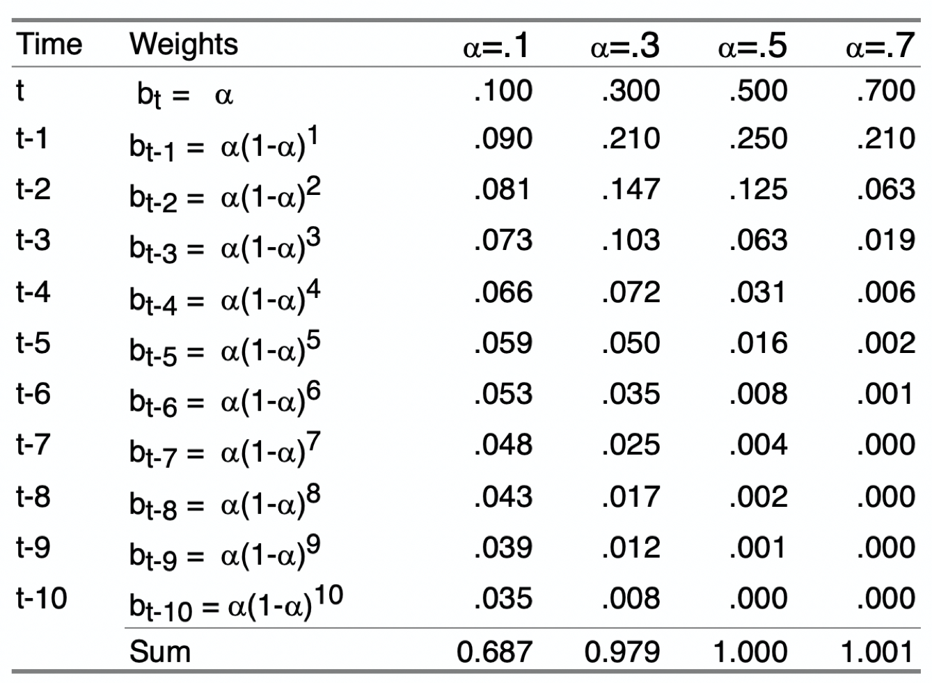
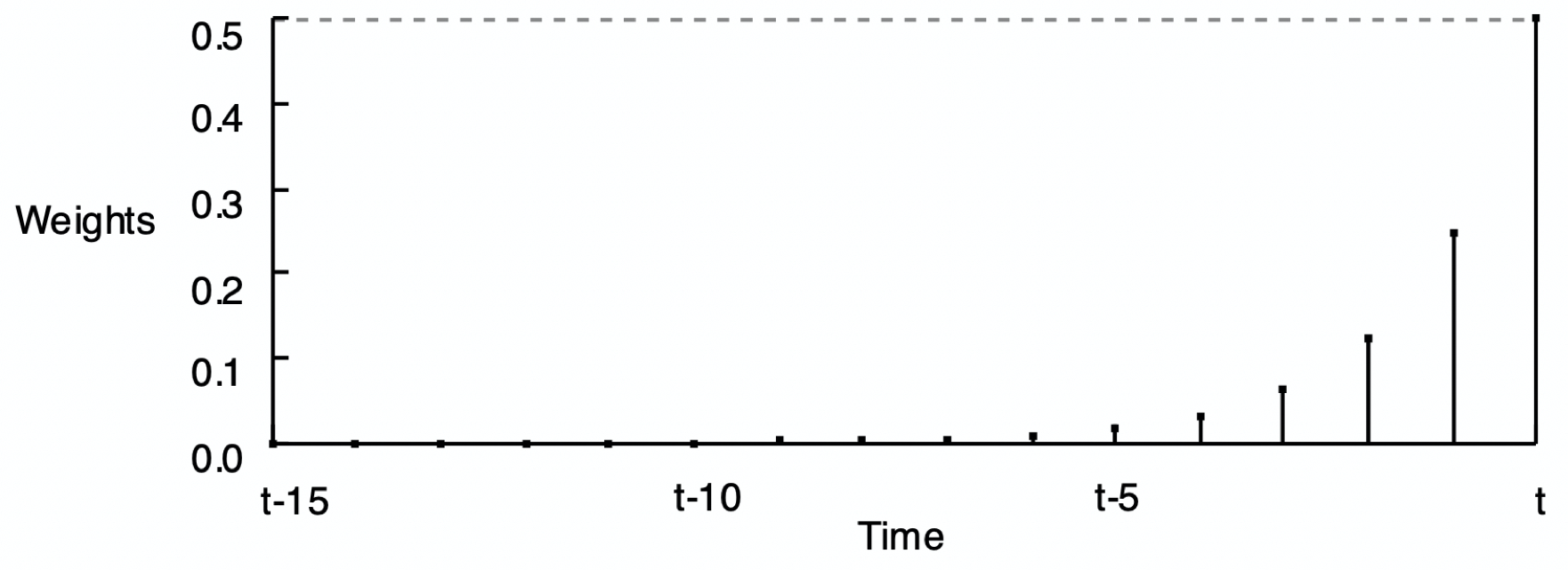
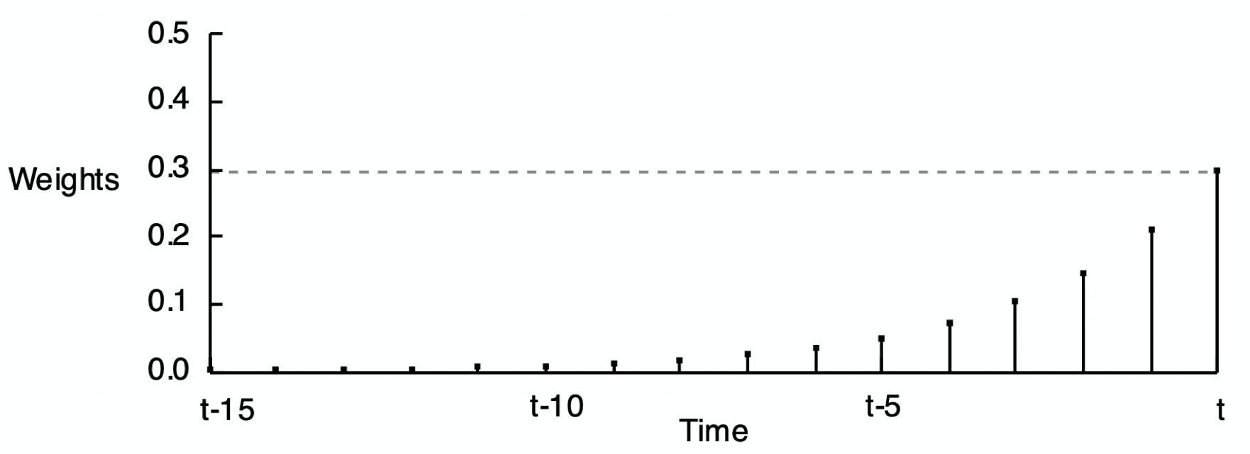
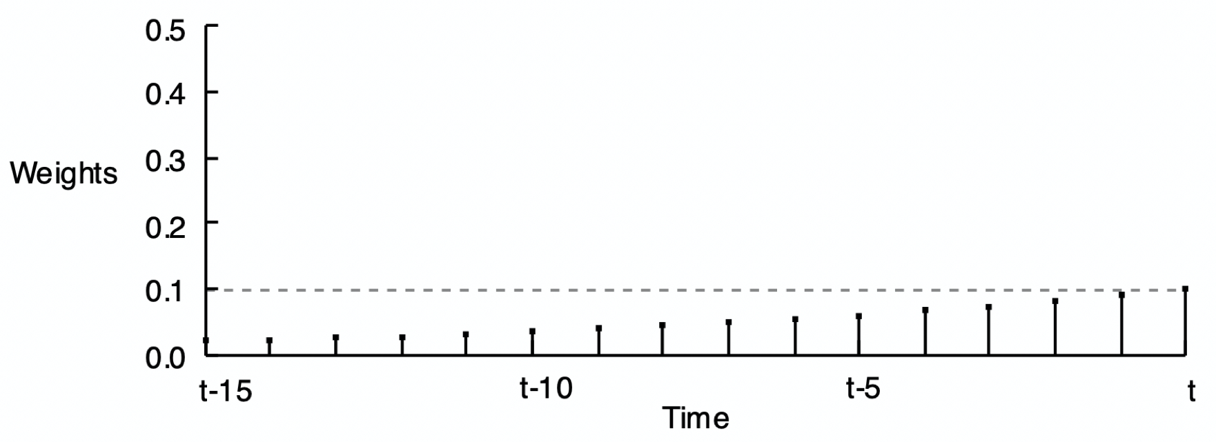
Figure 4.2 shows the pattern of weights for three different values of \(\alpha\). The reason for the word exponential in the name of this smoothing method is demonstrated by comparing Figure 4.2 (a), Figure 4.2 (b), and Figure 4.2 (c) according to their respective smoothing weights. Each set of weights in the following three figures exponentially decreases from the current time period back into previous time periods, but at different rates.
As stated, compute the forecast of the value of \(y\) at the next time period only according to the value of the current time period:
\[(\alpha) y_{t} + (1 - \alpha) \hat y_{t}\]
These weights across the previous time periods shown in Figure 4.2 are not explicitly computed to make the forecast but are implicit in the forecast. Their use would provide the same result if the forecast was computed from all of these previous time periods.
5 Implementation
5.1 Simple Exponential Smoothing
Refer to the previously described exponential smoothing model as simple exponential smoothing or SES. Applying the smoothing to the data yields a self-correcting model that adjusts for forecasts made from the beginning of the series through the latest time period.
Unfortunately, the simple exponential smoothing model, SES, with its smoothing parameter, \(\alpha\), has limited applicability. The procedure only correctly applies to stable processes, that is, models without trend or seasonality, a model with a stable mean and a stable variability over time.
Regardless of the form of the time series data, simple exponential smoothing provides a “flat” forecast function, all forecasted values are equal.
This first example appropriately applies to the SES model with data characterized by a stable mean and a stable variability over time.
5.1.1 Data
To illustrate, first read some stable process data into the d data frame. The data are available on the web at:
http://web.pdx.edu/~gerbing/data/StableData.xlsx
d <- Read("http://web.pdx.edu/~gerbing/data/StableData.xlsx")
The lessR function Read() reads data from files in any one of many different formats. In this example, read the data from an Excel data file into the local R data frame (table) named d. The data are then available to lessR analysis functions in that data frame, which is the default data name for the lessR analysis functions. That means that when doing data analysis, the data=d parameter and value are optional.
The data represent monthly measurements of Variable Y3. Here are the first six rows of data.
head(d) Month Y3
1 2019-07-01 49.3042
2 2019-08-01 49.3760
3 2019-09-01 51.3605
4 2019-10-01 50.5292
5 2019-11-01 49.8766
6 2019-12-01 49.7658Before submitting a forecasting model for analysis, first view the data to understand its general structure.
Plot(Month, Y3)
Use the Plot() function because we are plotting points, which are by default for a time series connected with line segments.
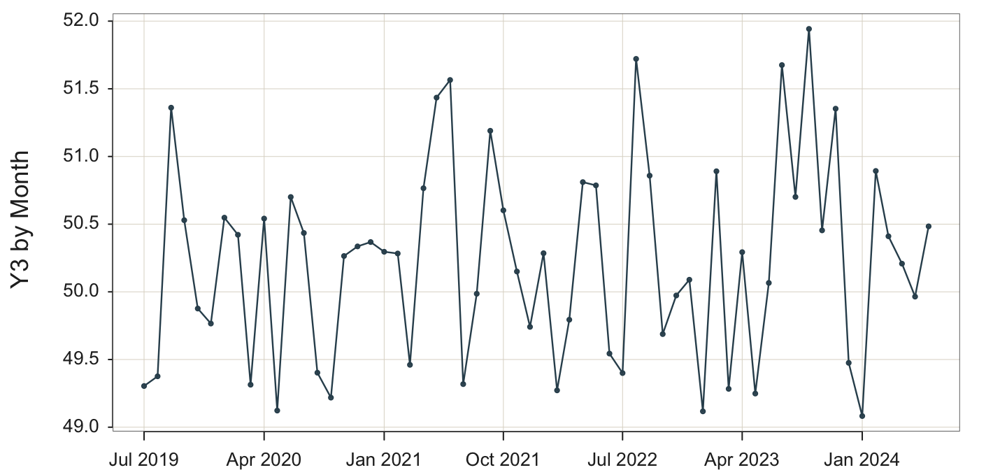
The visualization in Figure 5.1 apparently renders a stable system. There is no obvious trend, the fluctuations around the center are irregular without apparent seasonality, and the variability of the system appears to remain constant over time.
5.1.2 Decomposition
To more formally evaluate the characteristics of the time series for variable Y3, analyze the data with a seasonal and trend decomposition. Figure 5.2 shows the resulting visualization.
STL(Month, Y3)
STL() is the Base R function stl() with a color enhancement and provided statistics for assessing the strength of the trend, seasonal and error components of the time series.
When calling the function, specify the x-axis variable first followed by the y-axis variable.
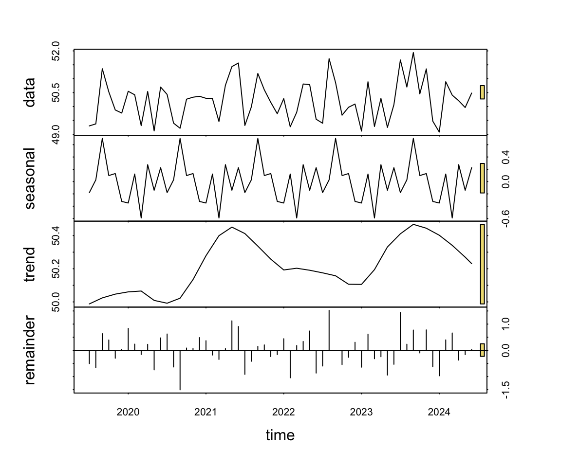
The visual output of the decomposition consists of four separate plots stacked over each other. The first plot is the data. The seasonal and trend plots follow, plus the extent of the unaccounted-for error called the remainder.
Regardless of the data analyzed, the seasonal and trend decomposition always identifies seasonality and trend. The question is if the effects that have been identified are sufficiently large to be meaningful. To answer that question, we have visual and statistical information.
The visual information for gauging the extent of a component’s effect is the gold bar at the extreme right of each of the four plots.
Each gold bar at the right side of each plot in the trend and seasonal decomposition visualization indicates the amount of magnification required to expand that plot to as large as possible to fill the allotted space. The larger the bar, the smaller the effect.
For example, the seasonal effect is virtually nonexistent because its corresponding bar is as large as possible given the size of the corresponding, narrow plot. Without that large magnification, the plot of the seasonal effect would be tiny.
The statistical output provides the values that reflect the size of the gold bars in terms of the proportion of variance of the variable accounted for by each component. The seasonality component accounts for only 3.0% of the overall variability of the data. Trend accounts for more, 19.9% but the dominant component is the error, 63.6%.
Total variance of Y3: 0.5498205
Proportion of variance for components:
  seasonality --- 0.199
  trend --------- 0.041
  remainder ----- 0.716
Although the trend shows a small effect in these data, it is likely a sampling fluke in this relatively small data set, particularly when compared to the random error effect. Notice also that the trend is composed of random appearing ups and downs. There is little consistent up or down across annual time periods.
We conclude that the process likely generates random variation about the center over time. The data further support this, demonstrating a constant level of variability.
5.1.3 Visualize the Forecast
Assuming a stable system, proceed by applying the SES forecasting model to the data.
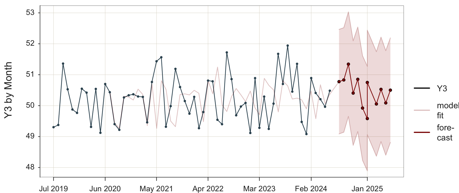
Plot(Month, Y3, time_ahead=8, es_trend=FALSE, es_season=FALSE)
Use the Plot() function because we are plotting points, which are by default for a time series connected with line segments . time_ahead: Indicate an exponential smoothing forecast by specifying the number of time units for which to do the beyond the last data value. By default, the forecast is based on an additive model.
es_trend: Trend parameter for an exponential smoothing forecast. Here, set to FALSE so as to not allow for trend.
es_season: Seasonality parameter for an exponential smoothing forecast. Here, set to FALSE so as to not allow for seasonality.
To specify a simple exponential, smoothing model, SES, set both es_trend and es_seasontoFALSE`.
The accompanying visualization in Figure 5.3 shows four separate visualizations:
- data: [black line] from which the model is estimated
- model fit: [light red line] the model’s fitted values to the data
- forecast: [dark red line] the model’s forecasted future data values
- 95% prediction interval [light red band about the forecasted values]
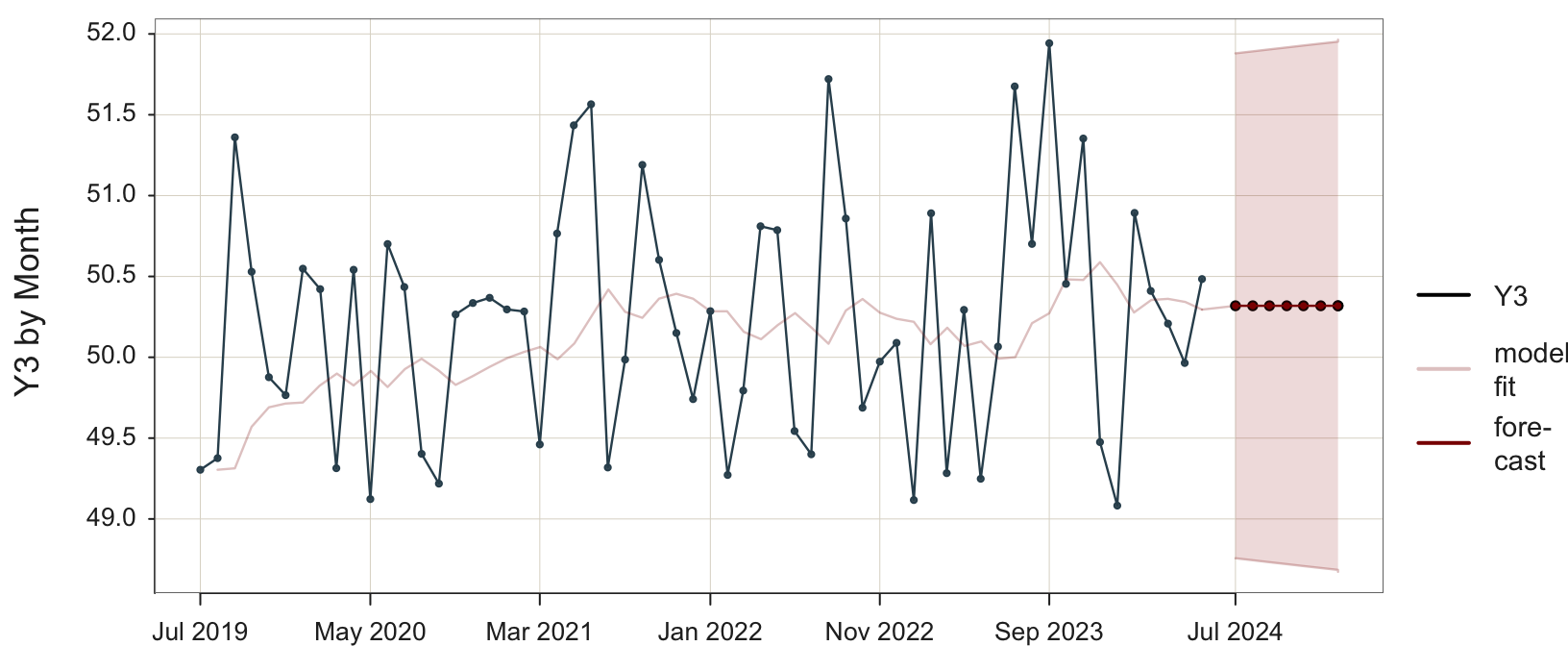
The forecasted values for the future time points are equal. The SES model forecasts the same value into the future. The large discrepancy between the data and the model’s fitted values indicates that the model does not adequately explain the variability in the data.
The time series of the fitted values in Figure 5.3 shows the smoothing effect of the exponential smoothing model applied to the training data. The model is applied to act as if forecasting the next data value in the time series from the previous value, even though both values have already occurred.
The first two data values are well below the center, so the fitted model begins with low values, increasing over time as the data values increase. After this initial recovery, the fitted values show no trend, but the model attempts to capture seasonality, which does not exist. After each particularly large observation relative to the rest, the fitted model increases, then decreases in value following a decrease in the data. Without any regular pattern of increasing and decreasing data, the ups and downs of the fitted model are also irregular.
Figure 5.3 also visualizes the 95% prediction interval for each forecast value.
Estimated range of values that contains 95% of all future values of forecasted variable \(y\) for a given future value of time.
For this SES model, the 95% prediction interval spans the range of the data. The confidence range grows increasingly larger for forecasted values further in the future.
To be more confident that the prediction interval will contain the future value of \(y\) when it occurs requires a larger prediction interval. At the extreme, for a data value that is in the range of this example, we would be approximately 99.9999999% confident the data value will fall within the range of -10,000 to 10,000.
5.1.4 Text Output
In addition to the visualization, the precise forecasted values are also available with their corresponding 95% prediction intervals along with other information. The text output of the analysis follows.
Sum of squared fit errors: 37.93357
Mean squared fit error:    0.65403

Coefficients for Linear Trend
 b0: 50.31855

Smoothing Parameters
 alpha: 0.12549

         predicted  upper95  lower95
Jul 2024  50.31855 51.88030 48.75680
Aug 2024  50.31855 51.89255 48.74455
Sep 2024  50.31855 51.90470 48.73240
Oct 2024  50.31855 51.91677 48.72034
Nov 2024  50.31855 51.92874 48.70836
Dec 2024  50.31855 51.94062 48.69648
Jan 2025  50.31855 51.95241 48.68469
Feb 2025  50.31855 51.96413 48.67297
The exponential smoothing software provides the value of \(\alpha\) for this minimization, which, for this analysis is \(\alpha\) = 0.125. Usually, the software allows for customizing the value of \(\alpha\), but the value computed by the software is often the recommended value to use. This value of \(\alpha\) results in the smallest value of RMSE possible for that version of the exponential smoothing model for that data. For example, setting \(\alpha\) at 0.2 results in a RMSE of 0.665. Increasing \(\alpha\) to 0.5 further increases RMSE to 0.771.
5.1.4.1 Forecasted Values
Find the forecasted values under the predicted column. For the SES model, the forecasted values equal one another.
\[\hat y_{2024.Q3} =\hat y_{2024.Q4} = \; ... \; = \hat y_{2026.Q2} = 50.319\]
As indicated, the simple exponential smoothing model only accounts for the level of the forecasting data, applicable only to data without trend or seasonality.
5.2 Problem with SES
5.2.1 Data
The flat forecast is appropriate for data without trend or seasonality, as illustrated in Figure 5.3 for a stable process. The problem arises when trend and/or seasonality are present in the data. Unfortunately, the simple exponential smoothing forecasts are “blind” to any trend and seasonality in the data. To illustrate, the following analysis begin with data described by trend and seasonality and then analyze that data with several different exponential smoothing models.
First, consider an SES model applied to the data with trend and seasonality in the data. The data are available on the web.
http://web.pdx.edu/~gerbing/0Forecast/data/SalesData.xlsx
d <- Read("http://web.pdx.edu/~gerbing/data/SalesData.xlsx")
The lessR function Read() reads data from files in one of many different formats. In this example, read the data from an Excel data file into the local R data frame (table) named d. The data are then available to lessR analysis functions in that data frame, which is the default data name for the lessR analysis functions. That means that when doing data analysis, the data=d parameter and value are optional.
The data represent quarterly measurements of the variable Sales. The dates are listed as individual days, with each date representing the first day of the corresponding quarter. The 16 lines of the data table follow, reported quarterly from the first quarter of 2016 through the last quarter of 2019.
d Qtr Sales
1 2016-01-01 0.41
2 2016-04-01 0.65
3 2016-07-01 0.96
4 2016-10-01 0.57
5 2017-01-01 0.59
6 2017-04-01 1.20
7 2017-07-01 1.53
8 2017-10-01 0.97
9 2018-01-01 0.93
10 2018-04-01 1.71
11 2018-07-01 1.74
12 2018-10-01 1.42
13 2019-01-01 1.36
14 2019-04-01 2.11
15 2019-07-01 2.25
16 2019-10-01 1.74STL(Qtr, Sales)
STL() is the Base R function stl() with a color enhancement and provided statistics for assessing the strength of the trend, seasonal and error components of the time series.
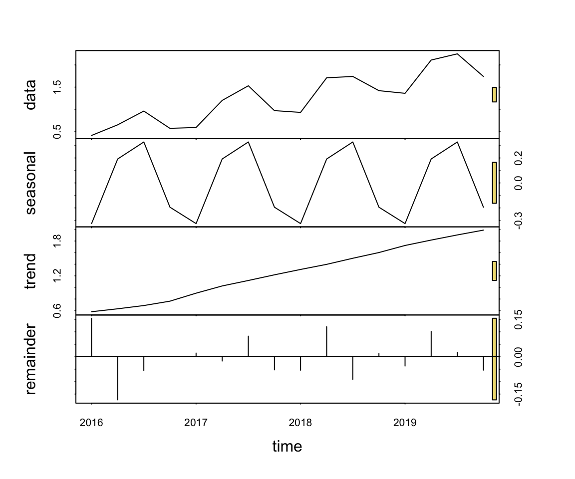
The data exhibit strong trend and seasonality.
Total variance of Sales: 0.318705
Proportion of variance for components:
  seasonality --- 0.241
  trend --------- 0.691
  remainder ----- 0.023
Figure 5.5 illustrates the unresponsive flatness of the forecast of a simple exponential smoothing model applied to time series data with trend and quarterly seasonality. The forecasted values capture neither the trend nor the seasonality inherent in the data.
Plot(Qtr, Sales, time_ahead=6, es_trend=FALSE, es_season=FALSE)
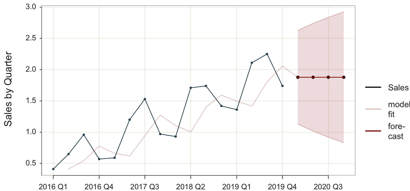
The poor fit of the SES model applied to these data is indicated by
- visualization: the discrepancy between the plot of the data values and the values fitted by the model
- statistic: the high value of MSE of 0.179
Visually, the lack of fit is indicated by the discrepancy of the data, the black line in Figure 5.5, compared to the fit of the model to the data, the light red line. Figure 5.5 shows the fitted data values lagging the actual data. For example, when the data peaks at a seasonal high point, the fitted values also increase as a proportion of the data but one time period later. The inherent seasonality in the data is reflected in fitted values with the lag, leading to less than optimal fit.
5.3 Forms of Exponential Smoothing
To adapt to structures other than that of a stable process, consider three primary components for modeling time series data: error, trend, and seasonality. There are two primary types of expressions for each of the three components: additive and multiplicative. Table 5.1 describes the general characteristics of the resulting six different types of models. The accompanying reading/video illustrates these models.
| Additive | Multiplicative | |
|---|---|---|
| Error | The average difference between the observed value and the predicted value is constant across different levels of the time series. The error does not depend on the magnitude of the forecasted value. | The average difference between the observed and predicted values is proportional to the level of the forecasted value. As the forecasted value increases or decreases, the error also increases or decreases proportionally. |
| Trend | The linear trend is upwards or downwards, growing or decreasing at a constant rate, which plots as a line. | The trend component increases or decreases at a proportional rate over time. The result is an upward sloping or downward sloping curve at an accelerating rate. |
| Seasonal | The intensity of each seasonal effect remains the same throughout the time series, adding or subtracting the same amount from the trend component along the time series. | The intensity of each seasonal effect consistently magnifies or diminishes, adding or subtracting a increasingly larger or smaller amount from the trend component along the time series. |
To generalize the simple exponential smoothing model to account for trend, add a trend smoothing parameter. While we will not delve into the formal definitions of these more complicated smoothing models, the concept of a smoothing parameter remains unchanged. However, the trend smoothing parameter applies to deviations from the slope derived from the data.
What type of model does your data support? As always, plot your data to visually discover any underlying structure. The problem is that the random noise that affects each data value obscures its underlying structure. Visualizing your time series allows you to see beyond the noise of any one data point and view the underlying structure as a whole. The better you understand the underlying structure, the more you can adjust the analytical forecasting technique to better match that structure.
5.3.1 Trend
To account for these deficiencies, the simple exponential smoothing model has been further refined to include additional smoothing parameters beyond the level of the time series, the \(\alpha\) (alpha) parameter.
Add a trend smoothing parameter to the model to account for trend in the data and the subsequent forecast.
This method provides for two smoothing equations, one for the level of the time series and one for the trend. As with the simple exponential smoothing model, the level equation forecasts as a weighted average of the current value, with weight \(\alpha\), and the current forecasted value with weight \(1-\alpha\). With this enhancement, however, the forecasted value is the level plus the trend.
Similarly, the trend gets its smoothing parameter, \(\beta\) (beta), which follows the same logic as the \(\alpha\) smoothing parameter. The trend, \(\beta\), is a weighted average of the estimated trend at Time t based on the previous estimate of the trend. The forecast now accounts for trend, as shown in Figure 5.6 of the trend and seasonal data.
For example, to specify a stable process model as in the previous example, specify the default model with additive errors, with no seasonality but allow for trend.
Plot(Month, Sales, time_ahead=6, es_season=FALSE)
time_ahead: Indicate an exponential smoothing forecast by specifying the number of time units for which to do the beyond the last data value. By default, the forecast is based on an additive model.
es_season: Seasonality parameter for an exponential smoothing forecast. Here, set to FALSE so as to not allow for seasonality.
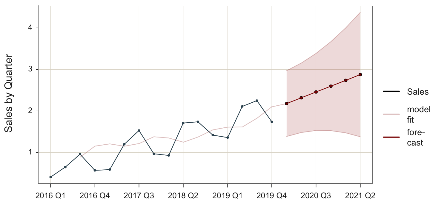
Although not listed in the output displayed here, the root mean squared error, RMSE is large: 0.179. To visualize the lack of fit, compare the black line for the data to the light red line with the fitted values. Enabling trend allows the fitted line to approximate the actual trend, but this model fails to account for the seasonality. Still, the forecasted values would likely be more accurate than those values obtained from the SES model. These forecasted values do extend the overall trend of the data.
5.3.2 Seasonality
Next, consider a model that explicitly accounts for seasonality but not trend with these data. Just as trend gets its smoothing parameter, so does seasonality, \(\gamma\) (gamma). The seasonality smoothing parameter, \(\gamma\), is a weighted average of the previous estimated corresponding seasonal periods. The forecast now accounts for seasonality, as shown in Figure 5.7 of the trend and seasonal data.
Because each seasonal period needs at least one corresponding previous seasonal data point, the fitted values begin well into the time series data. In this example, there are four quarters plus a leveling smoothing parameter, so the first fitted value is at the fifth time point, the first quarter of 2017.
Plot(Qtr, Sales, time_ahead=4, es_trend=FALSE)
time_ahead: Indicate an exponential smoothing forecast by specifying the number of time units for which to do the beyond the last data value. By default, the forecast is based on an additive model.
es_trend: Trend parameter for an exponential smoothing forecast. Here, set to FALSE so as to not allow trend.
To specify an additive model with no trend but allow for seasonality, only set es_trend to FALSE.
Sum of squared fit errors: 0.390
Mean squared fit error:    0.039

Coefficients for Linear Trend and Seasonality
 b0: 1.923
 s1: -0.302  s2: 0.186  s3: 0.299  s4: -0.183

Smoothing Parameters
 alpha: 1.000  gamma: 0.957

        predicted  upper95  lower95
2020 Q1   1.62000 1.903999 1.336001
2020 Q2   2.10875 2.510385 1.707115
2020 Q3   2.22125 2.713150 1.729350
2020 Q4   1.74000 2.307997 1.172003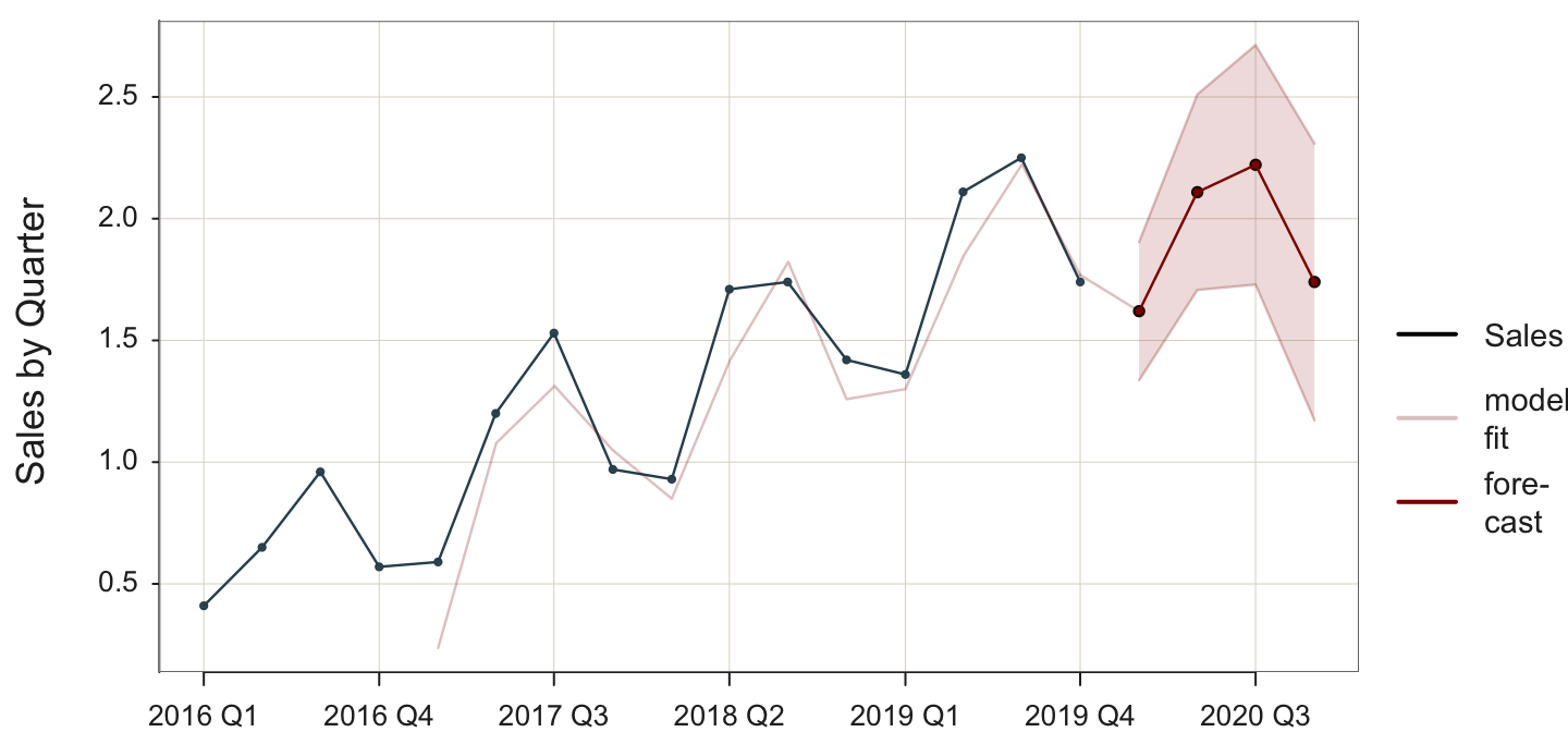
Again, the values are not displayed here. The mean squared error (MSE) for the model that does not account for trend but does account for seasonality reduces to 0.039 from the analysis of the previous models of this data. Examining Figure 5.7 reveals that the fitted values can capture seasonality even without formal specification. However, the fitted values still lag one time period behind the corresponding data values, contributing to the model’s lack of fit to the data.
Worse, the forecasted values must account for trend as the values are projected into the future. Without specifying seasonality, the model can still attempt to keep up with the seasonal ups and downs in the data, although lagging one-time unit. However, without specifying seasonality, projecting the data values into the future provides no ups and downs, for which the model can adjust. Instead, the model treats these ups and downs as random errors without the specification of seasonality. Accordingly, the forecast shows a repetition of more or less of the seasonal pattern but without any trend. When new data values collected in the future become available, a revised MSE can eventually be computed from the new data, which will be higher than the MSE for the training data.
The primary conclusion here is that if you observed trend or seasonality in the data, then a component present in the data should be accounted for in the model.
5.3.3 Trend and Seasonality
The data exhibit both trend and seasonality, so now analyze a more appropriate model that explicitly accounts for both characteristics.
Add a trend smoothing parameter and a seasonality smoothing parameter to the model to account for trend and seasonality in the data and the subsequent forecast.
This adaption to exponential smoothing is referred to as the Holt-Winters seasonal method. This method is based on three smoothing parameters and corresponding equations — one for level, \(\alpha\) (alpha), one for trend, \(\beta\) (beta), and one for seasonality, \(\gamma\) (gamma).
Apply the model to trend and seasonal data in Figure 5.8.
Plot(Qtr, Sales, time_ahead=4)
time_ahead: Indicate an exponential smoothing forecast by specifying the number of time units for which to do the beyond the last data value. By default, the forecast is based on an additive model.
Allow for trend and seasonality in the exponential smoothing forecast by not specifying the parameters es_trend and es_season, so the analysis begins at their default values with their corresponding optimal values estimated.
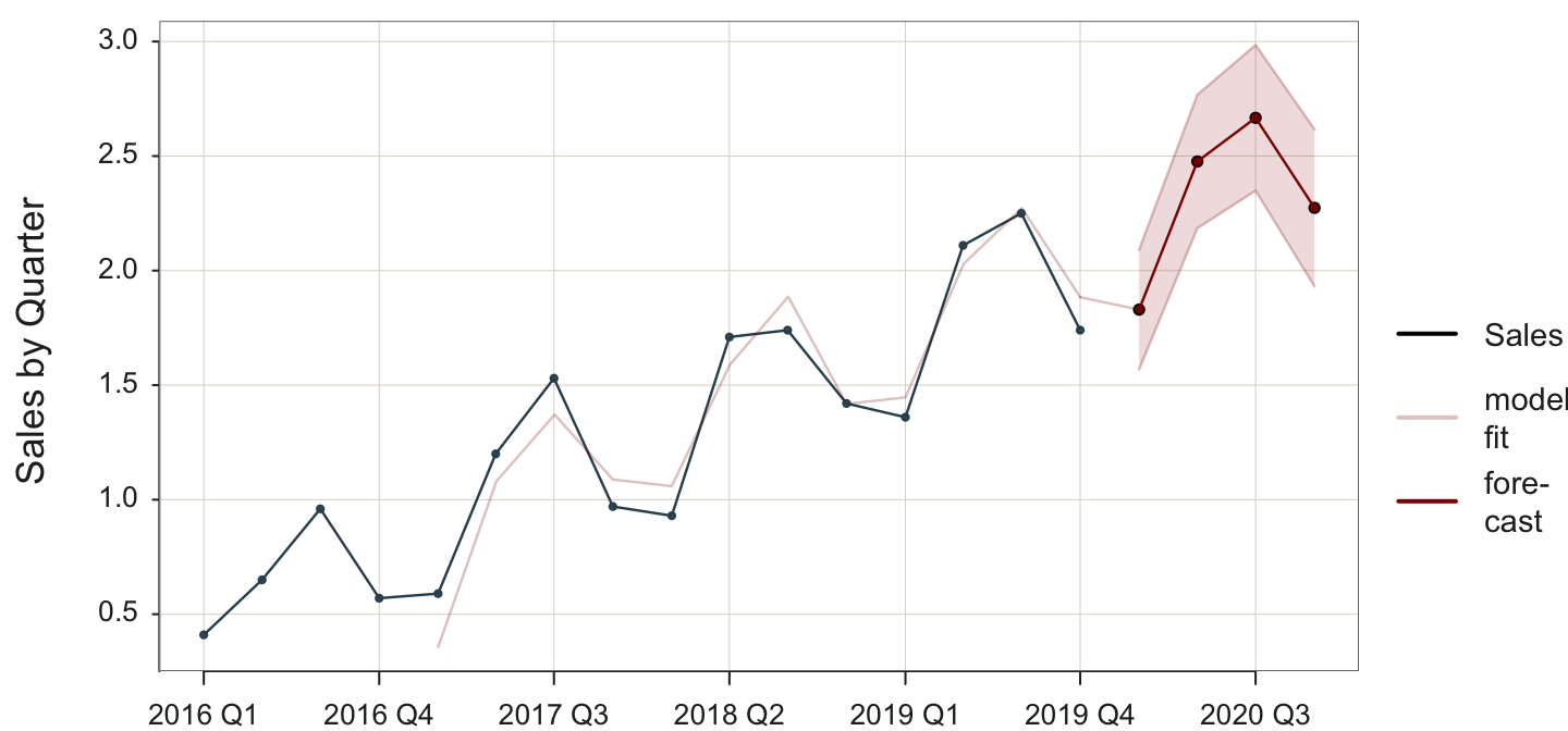
With this more sophisticated model both trend and seasonality extend into the future forecasted values. Accordingly, the fourth quarter tends to be lower in value than the previous quarters. Although there is increasing trend, Quarter #4 forecasted units are less than those forecasted for Quarter #3: \(y_{t+3}=\) 2.636 and \(y_{t+4}=\) 2.190.
This more general model accounts for the trend and the seasonality. Because the time series displays a regular pattern with relatively small random error, the forecasts show relatively small prediction intervals.
The precise fitted values and their corresponding prediction interval follow.
Sum of squared fit errors: 0.196
Mean squared fit error:    0.022

Coefficients for Linear Trend and Seasonality
 b0: 2.010  b1: 0.120
 s1: -0.300  s2: 0.227  s3: 0.297  s4: -0.215

Smoothing Parameters
 alpha: 0.492  beta: 0.000  gamma: 0.248

        predicted  upper95  lower95
2020 Q1  1.829643 2.090731 1.568555
2020 Q2  2.476363 2.767344 2.185382
2020 Q3  2.666898 2.984974 2.348821
2020 Q4  2.273926 2.616965 1.930887
The mean square error is the lowest of all the proposed models for the analysis of these data: MSE=0.022. This improvement is fit is apparent in the analysis of the data in Figure 5.8 compared to the light red line for model fit, which now more closely matches the data. In particular, the high peaks of each season match the corresponding peaks of the fitted model.
We can compare the fit of the different models, each to the same data with trend and seasonality, as in Table 5.2.
| Stable | Trend | Seasonality | Trend/Seasonality | |
|---|---|---|---|---|
| RMSE | 0.654 | 0.179 | 0.039 | 0.022 |
The more the form of the model matches the structure of the data, the better the fit to the training data and the more accurate are the forecasted values presuming the same underline dynamics that generate the data. Although we do not have an estimate of true forecasting error in this situation, the same logic applies. The more the data structure and model specification align, the more accurate the forecast of new data.
The output of these exponential smoothing forecasting analyses also includes the coefficients for linear trend and seasonality when relevant. The trend line for these data is estimated at Time t as
\[\hat y_{trend} = a + b (y_t) = 2.010 + 0.120 (y_t)\]
Each seasonality coefficient indicates the impact of the given season on the trend. A positive seasonality coefficient indicates and increase over the trend and a negative seasonality coefficient indicate a decrease. For example, the first coefficient is \(s_1\) = -0.300, so the first season is 0.300 units below the trend at that time value. Also, the second coefficient is \(s_2\) = 0.227, so the impact of the second season is to increase the value of trend by 0.227 units. The effect of each seasonality coefficient is additive, above or below the trend at that point.
Finally, the output of each exponential smoothing analysis includes the estimated value of the corresponding smoothing coefficients estimated in the analysis. The optimal coefficients for these data are \(\alpha\) = 0.492, \(\beta\) = 0.000, and \(\gamma\) = 0.248.
5.3.4 Overfitting
Why not just specify every model with trend and seasonality? Unfortunately, assessing the fit of a model on the data on which it trained is a kind of cheating.
The estimated model reflects too much random error in the training data that does not generalize to the new data for which the forecasts are made.
An overfit model, which detects excessive random noise in the data, can be misleading. The most crucial aspect of model evaluation is its performance on new data. In this context, the key question shifts from the model’s fit to the training data to its fit to forecasted data. If the model is overfit, the forecasting errors are likely larger than those from the training data.
For example, are the fluctuations in the time series data regular, indicating seasonality, or are they irregular, indicating random sampling fluctuations? Particularly for smaller data sets, not only can people see patterns where none exist over time, so can the estimation algorithm. It is possible to analyze data from a stable process and have the estimation algorithm indicate the presence of some seasonality. If this seasonality is projected into the future as a forecast, the forecasting errors will be larger if there is no seasonality in the underlying structure. A reasonable fit to the training data is not necessarily an advantage for reducing forecasting error.
Those seasonal fluctuations in the forecasted data values are an artifact of the sampling error inherited in the data on which the model trained. As shown in Figure 5.1, there is no seasonality inherent in these data.
Understand the properties of the time series data before constructing and analyzing an exponential smoothing forecasting model.
This is why it is important to understand the characteristics of the time series data before constructing a model and estimating its values from the data.
5.3.5 Multiplicity
Exponential smoothing models can be additive or multiplicative. Previously analyze models or additive. Here pursue a multiplicative model.
5.3.5.1 Data
To illustrate data with multiplicative effects, first read the data into the d data frame. The data are available on the web at:
http://web.pdx.edu/~gerbing/data/MultSeasonsData.xlsx
d <- Read("http://web.pdx.edu/~gerbing/data/MultSeasonsData.xlsx")
The lessR function Read() reads data from files in any one of many different formats. In this example, read the data from an Excel data file into the local R data frame (table) named d. The data are then available to lessR analysis functions in that data frame, which is the default data name for the lessR analysis functions. That means that when doing data analysis, the data=d parameter and value are optional.
The data represent monthly measurements of Variable Y. Here are the first six rows of data.
head(d) Month Y
1 2020-01-01 1.193951
2 2020-02-01 1.044351
3 2020-03-01 1.184061
4 2020-04-01 1.220409
5 2020-05-01 1.166378
6 2020-06-01 1.059063Before submitting a forecasting model for analysis, first view the data to understand its general structure, shown in Figure 5.10 for Variable Y.
Plot(Month, Y)
Use the Plot() function because we are plotting points, which are by default for a time series connected with line segments.
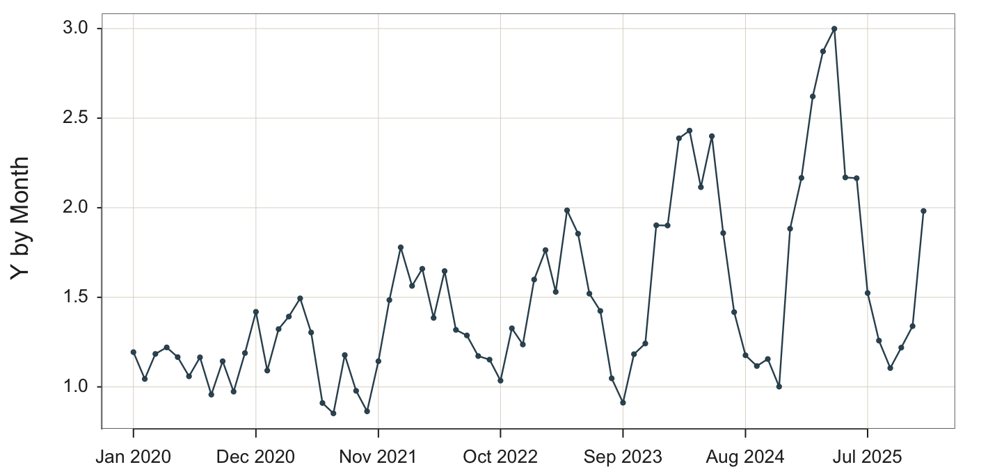
These data values unequivocally indicate multiplicative seasonality.
The seasonal fluctuations are proportional to the level of the time series, so that as the overall level of the series increases or decreases, the magnitude of the seasonal variations correspondingly increases or decreases.
The data indicate a regular pattern of seasonality but with a multiplicative effect. As time increases, the seasonal ups and downs increase as well.
5.3.5.2 Decomposition
The Base R stl(), on which the lessR function STL() is based, does not work with multiplicative seasonality and so is not applied here.
5.3.5.3 Visualize the Forecast
The necessity of the proposed exponential smoothing model that accounts for the multiplicity in the data is evident. A default additive model, which assumes a constant seasonality coefficient for each season, is not suitable for these data. The seasonal influence clearly grows over time, making a multiplicative model the most appropriate option. Attempting to analyze multiplicative data with an additive model will not yield as accurate results as with the proper multiplicative model. Additionally, the estimated seasonal coefficients will not be applicable as they are assumed to be constant for each season.
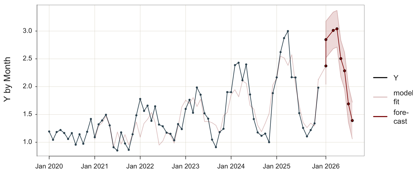
Analyze the data with the multiplicative model. The visualization appears in Figure 5.11.
Plot(Month, Y, time_ahead=10, es_type="multiplicative")
Use the Plot() function because we are plotting points, which are by default for a time series connected with line segments . time_ahead: Indicate an exponential smoothing forecast by specifying the number of time units for which to do the beyond the last data value. By default, the forecast is based on an additive model.
es_type: Set to "multiplicative" to specify a multiplicative model in place of the default additive model.
The statistical output follows.
Sum of squared fit errors: 3.8514589
Mean squared fit error:    0.0675695

Coefficients for Linear Trend and Seasonality
 b0: 1.8795577  b1: 0.0114368
 s1: 1.2546793  s2: 1.4962985  s3: 1.5735555  s4: 1.5792295  s5: 1.2933117  s6: 1.1730302
 s7: 0.8624606  s8: 0.7054201  s9: 0.6283890  s10: 0.6795133  s11: 0.7083866  s12: 1.0804782

Smoothing Parameters
 alpha: 0.0074537  beta: 1.0000000  gamma: 0.6597658

         predicted  upper95  lower95
Jan 2026  2.372592 2.701615 2.043568
Feb 2026  2.846605 3.175747 2.517463
Mar 2026  3.011578 3.340988 2.682167
Apr 2026  3.040498 3.370342 2.710655
May 2026  2.504811 2.834818 2.174804
Jun 2026  2.285272 2.615626 1.954918
Jul 2026  1.690091 2.020229 1.359953
Aug 2026  1.390420 1.720567 1.060272
In the multiplicative model with monthly data, the 12 seasonal coefficients represent seasonal factors that obtain the forecast by multiplying the level and trend components. These coefficients are multiplicative instead of additive. Each coefficient represents the relative effect of the corresponding month, interpreted in relation to the baseline of one, which indicates no change from the underline trend.
- Coefficient > 1: Season tends to be above the trend
- Coefficient < 1: Season tends to be below the trend
- Coefficient = 1: Season follows the trend exactly
For example, the first seasonal coefficient, for January, is \(s_1\) = 1.25. January typically has values 25% higher than the corresponding trend-level. If the trend for January forecasts 100 units, the forecast for January would be 125 units.
The coefficient for the seventh month, July, is below 1, \(s_7\) = 0.86. That is, July typically has values 14% lower than the corresponding trend. If the trend predicts 100 units, the forecast of the value of Y for July would be 86 units.
6 Appendix
Examining here only the \(\alpha\) smoothing parameter, the exponential smoothing model for the forecast of the next time period, t+1, is defined only in terms of the current time period t:
\[\hat y_{t+1} = (\alpha) y_t + (1-\alpha) \hat y_t\]
Project the model back one time period to obtain the expression for the current forecast \(\hat y_t\),
\[\hat y_t = (\alpha) y_{t-1} + (1-\alpha) \hat y_{t-1}\]
Substitute this expression for \(\hat y_t\) back into the model for the next forecast,
\[\hat y_{t+1} = (\alpha) y_t + (1-\alpha) \, \left[(\alpha) y_{t-1} + (1-\alpha) \hat y_{t-1}\right]\]
A little algebra reveals that the next forecast can be expressed in terms of the current and previous time period as,
\[\hat y_{t+1}= (\alpha) y_t + \alpha (1-\alpha) y_{t-1} + (1-\alpha)^2 \, \hat y_{t-1}\]
Moreover, this process can be repeated for each previous time period. Moving back two time periods from t+1, express the model is expressed as,
\[\hat y_{t-1} = (\alpha) y_{t-2} + (1-\alpha) \hat y_{t-2}\]
Substituting in the value of \(\hat y_{t-1}\) into the previous expression for \(\hat y_{t+1}\) yields,
\[\hat y_{t+1} = (\alpha) y_t + \alpha (1-\alpha) y_{t-1} + (1-\alpha)^2 \, \left[(\alpha) y_{t-2} + (1-\alpha) \hat y_{t-2}\right]\]
Working through the algebra results in an expression for the next forecast in terms of the current time period and the two immediately past time periods,
\[\hat y_{t+1} = (\alpha) y_t + \alpha (1-\alpha) y_{t-1} + \alpha (1-\alpha)^2 \, y_{t-2} + (1-\alpha)^3 \, \hat y_{t-3}\]