❝ All models are wrong, some are useful. ❞
A supervised machine learning analysis develops an equation called a model to predict the unknown. From a specific input value for one or more \(X\) variables, the prediction equation computes the corresponding predicted value for the target variable \(y\). There are many supervised machine learning methods for obtaining the prediction equation. This discussion focuses on the very first supervised machine learning method, regression analysis, which results in a linear prediction model.
The phrase regression analysis for predicting unknown values of a variable was created in the 19th century by a first cousin of Charles Darwin, Sir Francis Galton, one of the founders of social science. Modern machine learning procedures leverage considerably enhanced processing power with access to massive amounts of data. These developments enable previously unfeasible prediction algorithms beyond regression analysis. Nonetheless, understanding and doing supervised machine learning begins with regression analysis, which, in many circumstances, can produce as accurate a prediction as any machine learning method.
2.1 Linearity
The simplest and generally the most useful type of model is linear. Before we use regression to develop a linear supervised machine learning model, we first review some basic algebra of linear equations. The regression equations for prediction discussed here are linear equations, referred to as functions.
The model, the prediction equation, illustrates a central mathematical concept.
The prediction equation is an example of a function. More specifically, these equations model the relationship among the variables in the equation, so the equation is also called a model.
A concept introduced in middle-school algebra, a linear function, expresses \(y\) as the weighted sum of one or more \(X\) variables plus a constant. To express a linear function, we use a notation consistent with predictive models.
For a linear function of a single \(x\) variable, express the general form of the fitted value, \(\hat y\), as a weighted sum of the value of the variable \(x\) and a constant term.
The model relates variables \(x\) and \(\hat y\) in terms of a weighted sum given the weights \(b_0\) and \(b_1\). Define a specific linear function of one variable with specific numerical values of the weights \(b_0\) and \(b_1\). For example, \(b_0=5\) and \(b_1=7.3\) together define a specific linear function that computes the value of \(\hat y\) from a value of \(x\):
\[\hat y = 5 + 7.3(x)\]
Any other values for either or both of the weights, such as, \(b_0=2.93\) and \(b_1=-6.18\), define another linear function:
\[\hat y = 2.93 - 6.18(x)\]
Because multiple \(X\) variables can define a linear function, refer to the predictor variables generally with a capital \(X\). Reference any single \(X\) variable with a lowercase \(x\).
2.1.1 Slope
Represent a linear equation of one variable geometrically as a line. Plotting the paired values of \(x\) with \(\hat y\) computed from a linear function results in some type of a “straight surface”, no curves on the edges of the surface. For a model with two variables, here \(\hat y\) and a single \(x\), the plot is two-dimensional. A straight surface in two dimensions is a straight line.
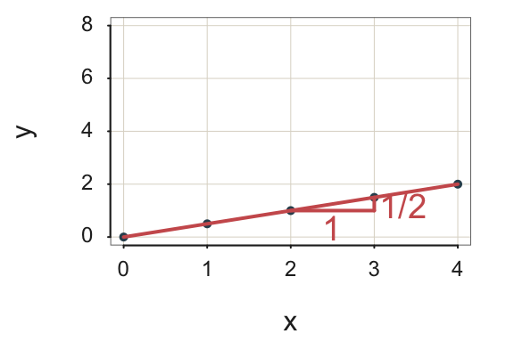
Example 1. Write the linear function with a slope of 0.5 and a constant term of 0 as: \[\hat y = 0.5 * x\]
To visualize the line, plot at least two pairs of points, connect the points with a line, and extend the line in both directions. The coordinates of each point on the line are a set of paired values of \(x\) and \(\hat y\). To identify a pair of points on the line, select some value of \(x\) and input into the equation to calculate the fitted value \(\hat y\). For example:
for \(x=2,\;\; \hat y=0.5*2 = 1.0\)
for \(x=3,\;\; \hat y=0.5*3 = 1.5\)
From these computations, plot the following two points, \(<2,1>\) and \(<3,1.5>\), to determine the line. As Figure 2.1 illustrates, each increase of one unit for \(x\) increases \(\hat y\) by the slope of \(b_1=\frac{1}{2}\), or \(0.5\) unit.

The result is a gently sloping line.
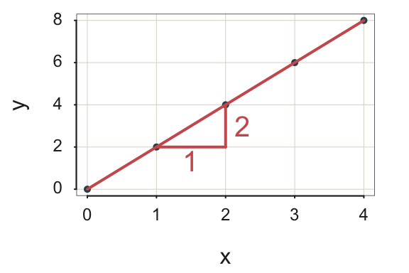
Example 2. In this next example, the slope is 2, again with the \(y\)-intercept of 0: \[\hat y = 2 * x\]
for \(x=1,\;\; \hat y=2*1 = 2\)
for \(x=2,\;\; \hat y=2*2 = 4\)
From these computations, plot the two points: \(<1,2>\) and \(<2,4>\).
Figure 2.2 shows that for each increase in \(x\) of one unit, the value of \(y\) doubles. A line with a slope of 2 is considerably steeper than from the previous example with a slope of 1/2.
Why do we care? To understand how \(y\) changes as a function of a change in \(x\) provides useful information for interpreting the model. For example, if interest rates rise by 1%, what is the predicted decrease in the number of purchased luxury automobiles?
2.1.2 \(y\)-intercept
A linear model contains a constant term, the \(y\)-intercept.
The intercept may be of interest, but typically not as much interest as the slope. In some contexts, the value of \(x=0\) is not even meaningful. For example, to predict a person’s Weight from their Height, a person with a Height of 0 makes no sense.
In the previous examples of \(y=\frac{1}{2}x\) and \(y=2x\), the \(y\)-intercept is 0, so it need not explicitly appear in these equations as the additive constant + 0.
2.2 Example Data
The feature variables and target variable of the model provide the data to estimate the model, the values of \(b_0\) and \(b_1\) for a linear model. For linear models with a single predictor variable, the data consist of the paired data values of feature \(x\) and target \(y\).
To learn the relationship between \(x\) and \(y\) requires using the computer to analyze existing data for both variables to estimate, that is, learn, the values of the \(y\)-intercept, \(b_0\), and the slope, \(b_1\), that relate \(x\) to \(y\) as well as they can be imperfectly related.
For example, an online clothing retailer needs the customer’s weight to size a garment properly. To learn the relationship between a customer’s weight and the size of the jacket that best fits the customer requires the weight and best-fitting size for many customers. The machine learns the relationship between the two variables from these paired data values of weight and size.
Once learned, the retailer applies this relationship when the customer’s weight is missing from the online order form. To better size a garment to fulfill an order, the retailer applies the model to compute an “educated guess” for the customer’s missing weight.
In practice, the analyst predicts the target variable, Weight, from multiple features and predictor variables. For simplicity, consider a model that predicts weight only from height and only for males to work with a one-feature model. The corresponding variable names listed in the data table are Height and Weight. Height is the \(x\)-variable, the feature or predictor variable, indicated by a lower-case \(x\) for a single variable. Weight is the \(y\)-variable, the target variable.
Consider a deliberately simple “toy” data set, which includes the height and weight of (only) 10 adult males randomly sampled from the retailer’s actual customer database. Table 2.1 shows some of the recorded data for these 10 customers, the same data from Figure 2.3.
| Height | Weight | |
|---|---|---|
| 1 | 64 | 115 |
| 2 | 68 | 160 |
| 3 | 67 | 145 |
| 4 | 74 | 200 |
| 5 | 61 | 146 |
| 6 | 66 | 175 |
| 7 | 71 | 180 |
| 8 | 70 | 145 |
| 9 | 68 | 173 |
| 10 | 69 | 210 |
Find the data on the web at http://lessRstats.com/data/regEg_data10.xlsx.
Different notation distinguishes two related but different concepts, the name of the variable and a data value for that variable.
For example, from the second row of the data table in Table 2.1, the person’s height is 68” with a weight of 160 lbs. Write these data values as \(x_2=68\) and \(y_2=160\). Subscripting the generic variable name with a specific variable name, such as \(x_{Height}\), references that variable. When a variable’s subscript is a number in this model with only one predictor variable, the reference is to a specific data value.
Enhance your understanding of the relationships inherent in the variables according to their data values by visualizing that relationship. Visualize the two columns of paired data from Table 2.1 with the scatterplot in Figure 2.3.
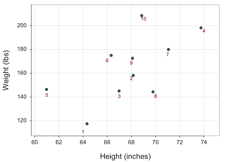
Each set of paired Height and Weight values in each row of the data table corresponds to a single point in the scatterplot of two dimensions. Refer to each of the paired data values in general as \(<x_i,y_i>\). In the following data visualization, the value on the horizontal or \(x\)-axis is the value of Height. The corresponding value on the vertical or \(y\)-axis is the value of Weight. Each plotted point represents the Height and Weight of a single individual, found in a single row of data.
The randomness inherent in the data imply that the data do not plot as a line. The points that represent data are scattered across the plot. The plot of the data values for \(x\) and \(y\) are scattered throughout the plot, hence the word: scatter.
As a data analyst, our goal is to discover the simplest functional form reasonably consistent with the data. The purpose of this function is to summarize the underlying relationship.
2.3 Model
2.3.1 Linear Form
Specify the general form of the model that relates the predictors to the target. Consistent with the shape of the scatterplot in Figure 2.3, a straight-line or linear model summary of the data appears appropriate.
\[\hat y_{Weight} = b_0 + b_1(x_{Height})\]
Assuming a linear relationship for these two variables, \(x\) and \(y\), we have two parameters in the model, the weights \(b_0\) and \(b_1\). From this general form of a model, derive a specific model, that is, from the data estimate specific values of \(b_0\) and \(b_1\). How do we estimate the values of these weights?
Regression analysis software applies this model to the data to learn the values of \(b_0\) and \(b_1\) that best describe the relationship in the data between the variables.
2.3.2 Analysis
2.3.2.1 Estimated Model
The analysis of the data values returns specific numeric values of the two weights, the slope and intercept, which then identifies a specific linear function for computing the value of \(\hat y\) from the value of \(x\). The equivalent geometric representation identifies a line through the scatterplot according to the values of the slope and intercept.
Analyze the data with regression analysis software to estimate the specified model from the data, such as with the free and open-source R or Python. Estimating the model is the machine learning how the predictor variable(s) relate to \(y\) by finding the optimal values of \(b_0\) and \(b_1\).
For these data values, here accomplish the regression analysis with the brief version of the Regression() function in the R package lessR (Gerbing 2021, 2023), reg_brief(). This function provides the easiest to use and most comprehensive regression analysis available in R or Python. Following standard R notation, the tilde indicates the specification of a model, with the response or target variable listed to the left of the tilde and the predictor variable(s) or feature(s) on the right. The Read() function that reads the data into R is also from lessR.
d <- Read("data/regEg_data10.xlsx")
reg_brief(Weight ~ Height)
The result for this example is the analysis of the linear model of a single \(x\) variable, Height, accounting for the value of a single \(y\) variable, Weight.
The output of the
Regression()function includes both the estimates of the model, slope and intercept as shown in Figure 2.4, much other statistical information, and data visualizations, such as the scatterplot with the regression line, as shown in Figure 2.5.
☞Identify the response or target variable and the predictor variable(s) or feature(s). Weight is the target or response variable, generically referred to as \(y\). Height is the feature or predictor variable, generically referred to as \(x\).
Identify the resulting estimated regression coefficients in Figure 2.4 from the output of the analysis of the linear regression model.

Regardless of the choice of software to accomplish the analysis, the output always includes what the machine learned. For the analysis of this model on this particular data set, the machine learned (estimated) the following values for the weights of the linear model:
- \(b_0\) = -171.152
- \(b_1\) = 4.957
☞Write the estimated regression model. \(\hat y_{w} = -171.152 + 4.957(x_{h})\)
2.3.2.2 Fitted Values
The estimated model provides the basis for computing the value fitted by the model, here \(\hat y_{Weight}\), for a given value of \(x\): From this estimated model, compute a fitted value of \(y\), \(\hat y\) from a given value of \(x\). If applying the model to new data where the value of \(y_i\) is not known, the fitted value, \(\hat y_i\), is the prediction of an unknown value.
☞ Show the calculation of the response or target value fitted by the model given the value of predictor variable Height, \(x_h = 66\) in.
\(\hat y_{w} = -171.152 + 4.957 (66) = 155.98\)
When the fitted value \(\hat y_i\) is calculated for all the rows of data, all the values of \(x\), the resulting plot of the paired values of \(x\) and \(\hat y\) is a straight line. Figure 2.5 visualizes this regression line is embedded in the scatterplot of the data, the paired value of \(x\) and \(y\). The figure also specifically focuses on the fitted value of \(\hat y=155.98\) given \(x=66\).
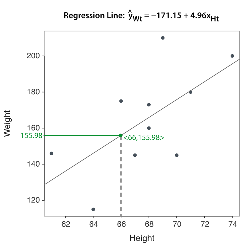
Visualize the estimated model as a line through the scatterplot of the data, as in Figure 2.5. For a given data value \(x_i\), distinguish between the corresponding data value \(y_i\) from the computed value of \(\hat y_i\) from entering the value \(x_i\) into the model.
Each regression analysis begins with the same sequence of steps common to all forms of supervised machine learning:
- Access the data values for variables \(x\) and \(y\) organized as a table
- Do the regression analysis from the data to estimate the model weights, here \(b_0\) and \(b_1\)
- From the estimated model: Calculate \(\hat y_i\) from a given \(x_i\) of interest
2.3.2.3 Slope Coefficient
Our estimated regression model provides a means by which to predict a person’s weight from their height. Indeed, prediction is one of the two primary goals of building a supervised machine learning model, such as with regression analysis. A complementary goal is understanding the relationship between the predictor variable(s) and the target being predicted. That understanding follows from interpreting the meaning of the estimated slope coefficient. And that meaning applies the definition of slope in any linear equation, apart from regression analysis per se.
The meaning of slope coefficient \(b_1\) contributes much to our understanding of the relationship between the variables \(x\) and \(y\).
Slope coefficient, \(b\), relating to fitted value \(\hat y\): Indicates exactly how much \(\hat y\) changes as \(x\) increases by one unit.
Slope coefficient, \(b\), relating to data value \(y\): Indicates how much \(y\) changes, on average, as \(x\) increases by one unit.
How much, on average, does weight increase for each additional inch of height for these specific data values from which the model was estimated?
☞Interpret the estimated (sample) slope coefficient. Applied only to this specific sample, on average, each additional inch of height results in an additional 4.957 lbs of weight.
In our interpretation, we specify on average because the data, the people’s weights do not fall exactly on the regression line. Height suggests but does not determine weight. Instead, for each height, weights vary about the predicted value that lies on the line.
Consistent with the definition of statistics as the analysis of variability, describing the extent of that variability is a key aspect of regression analysis, discussed shortly. The less variability, the less scatter, of the residuals for each value of \(x\), the better.
The estimated slope coefficient and \(y\)-intercept, however, are characterized by a pervasive, rather severe limitation. The estimated values of \(b_0\) and \(b_1\) are sample estimates. These values only describe how \(x\) relates to \(y\) in this particular data sample.
However, our concern is always how the relationship exists beyond the one sample from which the model was estimated. The full interpretation of these estimates follows from an application of statistical inference, obtained from the information in the remaining columns of Figure 2.4 beyond the Estimate column. This information allows us to generalize the sample estimates \(b_0\) and \(b_1\) to their corresponding likely values in the population, from which the data were sampled.
When interpreting the results of any data analysis, always specify if your conclusions are limited to the available sample data or if you are generalizing to the entire population from which the sample was obtained.
How are the estimated \(y\)-intercept and slope obtained from the analysis of the data values for the variables of interest? That topic is explained next.
2.4 Residuals
How to choose the line that runs through that scatterplot that best summarizes the data? How does the machine learn by choosing the optimal values for the weights \(b_0\) and \(b_1\)?
2.4.1 Variability
The key to understanding the process of choosing the optimal weights for the model begins with the definition of statistics.
The term variability, as used here, pertains to both the variability of the values of a single variable and, more generally, the co-variability of two or more variables. To assess variability inherent in the data values of a single variable, examine the deviation of each data value from a corresponding reference such as a mean. Regarding data analysis that involves the applications of statistics to numerical variables, understanding the results of these analyses requires understanding the concept of a deviation score.
Almost all data analysis of numerical variables, including regression models, involves the analysis of deviations, the distance a data value lies from some target value, the value fitted (computed) from a model applied to the predictor data value.
When applying the analysis of deviations to regression analysis, the deviations of interest are the residuals. The deviation for each row of data is the difference between what occurred, \(y_i\), and what the model indicates should have occurred, \(\hat y_i\).
2.4.2 Definition
The underlying concept is intuitive: Smaller residual errors indicate better fit. If the data values of the target variable are all close to their predicted target value, \(\hat y_i\),, the deviations of the data values from that target are small by definition. At the extreme, if all deviation scores are 0, then all the data values \(y\) are the same value, with no variability about the predicted target value \(\hat y\). On the contrary, if many deviations from the predicted target are large, then the data values are widely dispersed, indicating much variability.
A necessary requirement of a successful model is that the actual values of the target variable in the data, \(y_i\), tend to be reasonably close to the corresponding value of the target computed (fitted) by the model, \(\hat y_i\).
Does the model successfully recover the data? If so, the values of the target variable tend to be close to their corresponding values computed (fitted) by the model. If not, the values of the target variable in the data are relatively far from the values computed by the model.
From the estimated model, for any row of data from the data table, the \(i^{th}\) row, calculate a fitted value, \(\hat y_i\), from the corresponding data value \(x_i\). To compute a residual for a given value of predictor variable \(x\) we need both a data value for target variable \(y\), \(y_i\), and the corresponding value fitted by the model, \(\hat y_i\).
☞ Calculate the residual where for the sixth row of data, where \(y_6=175\) and the corresponding fitted value was previously calculated as \(\hat y_6 = 155.978\).
\(e_6 = y_6 - \hat y_6 = 175 - 155.978 = 19.022\)
Figure 2.6 visualizes the relation between the data value in the sixth row of \(y_6=175\), the fitted value of \(\hat y_6=155.978\), and the residual of \(e_6=19.02\).
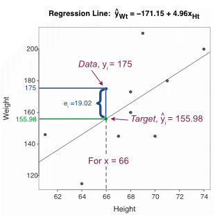
Unlike this toy data set, different customers in a data set of reasonable size likely share the same height, such as an \(x\) value for a height of 66 inches. Unfortunately, the model does not perfectly describe the data: Different people of the same height of 66 inches generally have different weights, which results in different residuals. A scatterplot instead of a line describes the data.
Why are residuals important? For all supervised machine learning algorithms, the residual is the key to how the machine learns the relationship between the variables. Learning relationships means choosing values of the model’s weights to minimize the size of some function of the residuals, here the minimization of the squared residuals. Better to choose a model that has relatively small residuals so as to minimize the unexplained scatter about the line.
The existence of the residual implies that a data value, \(y_i\), for target variable \(y\), consists of two components:
- explained by the model given \(x_i\), the target, the corresponding point on the line, \(\hat y_i\)
- unexplained, the residual, \(e_i\), the discrepancy of the data value of the target variable, \(y_i\), from the target, \(\hat y_i\)
Figure 2.7 illustrates this decomposition of a linear model for the data value \(y_i\) into a component that is accounted by the model, that is, understood by us who construct the model, and a component for which the model cannot explain. The model itself offers no insight into the reasons for the deviance, \(e_i\), of any one data value, \(y_i\), from the fitted value, \(\hat y_i\).
The residual variable, \(e\), likely results, in part, from many small, random perturbations such as those that lead to a fair coin flipped 10 times resulting in 6 heads instead of 5. The residuals may also result from important variables that are not present in the model. Regardless, the analysis of the composition of the \(e\) requires consideration of factors beyond the model itself.
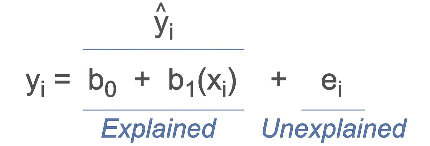
The data value of \(y_i\) that occurred is equal to the fitted value plus the residual, the error, from which \(y_i\) deviates from the fitted value, the point on the regression line.
2.4.3 Least-Squares
The machine (more precisely, the underlying estimation algorithm programmed on the machine) discovers the best-fitting line from an analysis of these residuals. A residual is calculated for each row of data. For linear regression analysis, the machine chooses the model’s weights to learn the relationship between \(x\) and \(y\) that minimizes the sum of the squared residuals. The residuals always sum to zero, so the minimization applies to the squared residuals.
Far from being a recent invention, what would later be called supervised machine learning in the form of the first least-squares analysis, was published well more than two centuries ago, 1805, by the French mathematician Adrien-Marie Legendre, who wrote (Smith 1929):
❝ I think there is none more general, more exact, and more easy of application, than … rendering the sum of the squares of the errors a minimum. By this means there is established among the errors a sort of equilibrium which … is very well fitted to reveal that state of the system which most nearly approaches the truth.❞
A primary distinction between Legendre’s work more than two centuries ago and our work today is that we are able do sophisticated least-squares analysis on very large data sets on our personal computers in a fraction of a second. For Legendre to analyze the data could require days of manual calculations on only relatively small data sets and impossible in a practical sense on any large set. Legendre did not call the estimation process of \(b_0\) and \(b_1\) machine learning because there were no machines to do the learning. Instead, the learning was accomplished by manual labor.
Applied to our predicted weight from height example, the least-squares estimation algorithm chose the weights \(b_0\) = -171.152 and \(b_1\) = 4.957. The resulting linear model minimizes the sum of the squared residuals (or errors), abbreviated as SSE.
Unlike most other machine learning estimation methods, we can solve directly for the optimal weights of a linear model evaluated according to the least-squares criterion.
The regression analysis functions, such as provided by R, Python, and many other software systems, including Excel, solve these equations to obtain the optimal weights for the data. Here optimal means minimizing the sum of squared errors or residuals.
Table 2.2 illustrates calculating the squared residuals for this one optimal solution. First, from the model with the estimated values \(b_0\) = -171.15 and \(b_1\) = 4.96, calculate the fitted values \(\hat y_i\), labeled as the variable FitWeight in the table. Then calculate the residual for each row, \(y_i - \hat y_i\). Next, square each residual, \((y_i - \hat y_i)^2\), labeled as the variable ResSq in the table.
| Customer | Height | Weight | FitWeight | Residual | ResSq |
|---|---|---|---|---|---|
| C00344 | 64 | 115 | 146.065 | -31.065 | 965.034 |
| C12965 | 68 | 160 | 165.891 | -5.891 | 34.704 |
| C18805 | 67 | 145 | 160.935 | -15.935 | 253.924 |
| C25180 | 74 | 200 | 195.630 | 4.370 | 19.097 |
| C26364 | 61 | 146 | 131.196 | 14.804 | 219.158 |
| C34263 | 66 | 175 | 155.978 | 19.022 | 361.836 |
| C36086 | 71 | 180 | 180.761 | -0.761 | 0.579 |
| C39288 | 70 | 145 | 175.804 | -30.804 | 948.886 |
| C44030 | 68 | 173 | 165.891 | 7.109 | 50.538 |
| C45149 | 69 | 210 | 170.848 | 39.152 | 1532.879 |
Sum the values in of the squared residuals in the ResSq column in Table 2.2 to obtain the sum of squared errors or SSE, \(\Sigma e_i^2\). This value, SSE, is the value minimized by the estimation algorithm. Find this optimized value from the output of a regression analysis in the Analysis of Variance (ANOVA) table, as in Figure 2.8. This example lists the Sum of the Squared Residuals as 4386.674.

The result: \(\Sigma e_i^2\) = 4386.64. You can develop a simple worksheet such as with Excel to mimic the form of Table 2.2 and plug in any other values for \(b_0\) and \(b_1\) to obtain the fitted values, residuals, and squared residuals. However, any other \(b_0\) or \(b_1\) values result in a sum of squared errors exceeding the obtained 4386.64.
2.4.4 Gradient Descent
Most machine learning methods, however, are not amenable to direct solution.
The following material, from the data and calculations in Table 2.2, illustrates the application of the gradient descent method to the minimization of the sum of squared errors. Although software for regression analysis provides an analytical solution, applying an intuitive gradient descent method illustrates the method and further enhances the meaning of the sum of squared errors or residuals.
video [7:05]: Meaning of the Sum of Squared Errors Fit Criterion.
pdf document: Written contents of the video.
Excel worksheet: Used to construct the example in the video.
As the video and related material illustrate, every set of values for the weights yields a corresponding sum of squared errors, SSE. However, only one set of weights, the least-squares solution for \(b_0\) and \(b_1\), provides the minimum possible SSE for that specific data set.
2.5 Model Fit
Supervised machine learning models, such as linear regression, predict unknown values of a target variable of interest. An essential question that must be answered after estimating the model is how well does the model predict these unknown values? Do these fitted values tend to be close or far away from the actual value of the target variable when it is known?
The geometric expression of building a linear model for prediction is placing a best-fitting line through the scatterplot of the \(x\) and \(y\) data values. However, a line can be placed through any scatterplot and that line (model) may or may not be useful for prediction. The line could indicate a good fit, with the points in the data scatterplot tightly clustered about the sloped line. Or, the best-fitting line that minimizes SSE could indicate a poor fit, with the scatterplot points spread widely about the line, displaying large residuals. “Best” is not necessarily “good”.
Doing machine learning involves testing different models in search of the model that yields the most accurate predictions, models in which the data values most closely equal the target values specified by the model. To begin, evaluate the model’s fit on the training data, the data on which the model trained.
A model must fit the data on which it was estimated (trained) reasonably well before proceeding with evaluating the model for its ability to predict on new data, where \(y\) is not known.
How to compare fit of models across different data sets? Across different models? Fit is all about the size of these deviations, the residuals or errors, whether testing fit on the training data or on new data. To assess the size of the residuals in a least-squares regression analysis, examine the sum of the squared residuals. The algorithm chooses regression model weights \(b_0\) and \(b_1\) that minimize the sum of the squared errors, abbreviated SSE, across all the rows of data from which the model was estimated.
\[\begin{align*} SSE &= \Sigma e_i^2 \\ &= \Sigma (y_i - \hat y_i)^2 \end{align*}\]
Much of data analysis is about the analysis of deviations of individual data values from some target, usually a mean, \(y_i - \hat y_i\). The mean could be of all the data, or, for regression models, the mean of the data about a specific point on the regression line for a given value of \(x\). To understand data analysis, understanding expressions such as \(\Sigma (y_i - \hat y_i)^2\) is essential.
For our toy data example of forecasting weight from height, \[SSE = 4386.674\] However, SSE is not the value directly used to evaluate and compare fit across models and data sets. Instead, we leverage this statistic to derive two useful fit indices for comparing fit across different models, explained next.
- standard deviation of the residuals
- \(R^2\)
Both of these fit indices follow directly from the SSE equal to \(\Sigma e^2_i\).
2.5.1 Standard Deviation of Residuals, \(s_e\)
Model fit indices follow directly from the minimized sum of the squared errors, SSE or \(\Sigma e_i^2\). By itself, however, this sum is not the most interpretable indicator of fit. The size of a sum of positive numbers, such as SSE, depends on the number of values that contribute to the sum. A model estimated from a larger data set would generally have a larger \(\Sigma e_i^2\) than the same model estimated from a smaller subset of the same data. The larger data set has more rows of data and so contains more positive, squared numbers to sum. The more positive numbers are summed, the larger the sum. To eliminate this sample size effect of a sum, convert the sum to the corresponding mean.
2.5.1.1 Degrees of Freedom
In many statistical analyses, however, when computing an average we do not divide by the sample size, \(n\), but rather by a slightly reduced \(n\), such as, in this example, \(n-2\). What is the basis of this \(n-2\)? To calculate the mean of the squared error scores, we first need the error scores. To calculate the errors, we first need to pass through the data to estimate the weights \(b_0\) and \(b_1\). After this first pass through the data to estimate the model, we then use the estimated values \(b_0\) and \(b_1\) to do a second pass through the same data to calculate the error score, \(e_i\), for each row of data.
Knowing values of \(b_0\) and \(b_1\) calculated from \(n\) rows of data implies that if we also know the values of \(n-2\) error scores, we can calculate the values of the remaining two error scores. This second pass through the data effectively reduces the number of values free to vary from \(n\) on the first pass to \(n-2\) on the second pass.
Calculate the mean of a statistic based on its degrees of freedom when there is a second pass through the same data that uses statistics calculated from the first pass.
With any decent sized sample, particularly a big data sample with \(n\) well over a thousand if not tens of thousands or more, there is no practical impact of computing an average by dividing by \(n\) or \(n-2\). For example, a huge sum of squared errors from a sample of \(n=93,146\) will convert to the same mean within many digits of decimal precision if dividing SSE by \(93,146\) or \(93,144\).
Still, in small samples, dividing by \(n\) rather than \(n-2\) may noticeably impact the fit index. Comparing fit of different models on the same data set does not depend on which number appears in the divisor because all models are based on the same sample size.
2.5.1.2 Mean Squared error
The mean of the squared errors is more appropriate than their sum for assessing fit. In other words, take the mean of squared errors instead of their sum.
For regression analysis with a single predictor, \(df=n-2\) for \(n\) rows of data. In this example, calculate MSE with SSE and its degrees of freedom, \(df=10-2\), also found in the ANOVA output from a regression analysis, such as in Figure 2.8.
\[\textrm{MSE} = \frac{SSE}{df} = 548.334 = \frac{4386.674}{8}\]
The MSE works well to compare the fit of different models, and is reported in many different analyses and by different software applications. However, there is one issue of interpretability that can be further developed.
2.5.1.3 Define
The unit of a mean square is the squared units of the original measurements. As with the computation of the standard deviation in general, further transform the MSE back to the original unit of measurement with the square root.
Much if not most data analysis, including supervised machine learning with regression analysis or any other machine learning technique, is based on the concept of the standard deviation. To understand more regarding this essential, core concept of data analysis, reference the following pdf and video [16:37]. An excerpt extracted from that pdf, expands the definition of the standard deviation step-by-step as found in the video.
1 Many texts refer to \(s_e\) as the standard error of estimate. More straightforward to refer to \(s_e\) as the standard deviation of the residuals, which is its definition.
Taking the square root allows the expression of the fit index with, for example, pounds of weight instead of squared pounds.1 In this example:
\[s_e = \sqrt{MSE} = \sqrt{548.334} = 23.417\]
The point on the regression line for a given value \(x_i\) is the specific target value, \(\hat Y_i\). Because the residuals about each \(\hat y_i\) typically follow a normal distribution, we can rely upon normal curve probabilities to understand the extent of \(s_e\). A normal distribution has 95% of its values within 1.96 standard deviations of its mean. Given the assumption of normality, a range of just under four \(s_e\)’s contains about 95% of the residuals about any given point on the regression line, \(\hat y_i\).
\(s_e\) summarizes the amount of scatter about each point on the regression line.
Directly visualize the amount of scatter about the regression line for a given value of \(x\) as shown in Figure 2.9. Here the scatterplot is of the small data set from which the model was estimated. For the value of the arbitrarily chosen \(x=68\), the corresponding fitted value is \(\hat y=166.13\).
Typically, all the values of \(y\) for a given value of \(x\) are normally distributed about \(\hat y\). For this analysis of this small data set, however, there are only two values of \(y\) for \(x=68\). Although these two values are sampled from a presumably normal distribution, we cannot directly visualize the normality of the full distribution. We can, however, draw the normal curve that would be demonstrated with enough data.
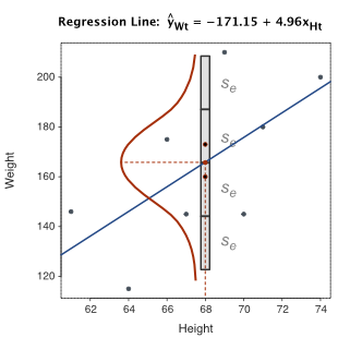
A much larger data set more precisely illustrates the range of variation of the residuals about each point on the regression line, with many values of \(y\) about \(\hat y=161.13\) just for values of \(x=68\). Find such an example in Figure 2.10 from several thousand rows of data with Height, \(x\), measured to the nearest inch, many of them \(68\) inches tall.
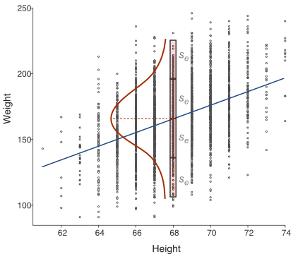
All of these values in Figure 2.10 directly demonstrate a normal distribution. Most values of \(y\) are close to \(\hat y=166.13\). Applying normal curve probabilities, only about 5% of the values lie more than about two standard deviations away from \(\hat y=166.13\) (1.96 standard deviations to be precise).
The larger \(s_e\), the larger the scatter about the line. What is the range of the scatter? Given that 95% of the values of a normal distribution lie within 1.96 standard deviations of the mean, about 95% of the values scattered about each point on the regression line lie within a range of just under \(4s_e\), illustrated in Figure 2.9 and Figure 2.10 for \(x=68\).
All regression analysis software reports the value of the standard deviation of the residuals, \(s_e\). The output below is from the lessR (Gerbing 2021) function Regression() for the example toy data set from Table Table 2.2. The output includes the value of \(s_e\) as well as the 95% range of variation about each point on the regression line, assumed at the same level of variation across the values of \(x\).
Standard deviation of Weight: 28.529

Standard deviation of residuals:  23.417 for df=8
95% range of residuals: 107.997 = 2 * (2.306 * 23.417) ☞Evaluate fit with the standard deviation of residuals, \(s_e\). \(s_e\) describes the amount of variation about the regression line, assumed the same general level of variability for each value of \(x\). In this analysis, \(s_e= 13.681\). This value is fairly large, given that the 95% range of variation about each value of \(x\) on the regression line is approximately \(4\) times \(s_e\), or almost \(108\) lbs.
The amount of scatter shows how much error exists in the best case scenario in which we optimized the model for the one specific data set from which the model is estimated. The smaller the variation about the regression line, the better, but how to interpret the size of the range of residual variability? Compare the scatter about the line2 of \(y\) for each value of \(x\) to the extent of the overall variation of \(y\) about the mean of \(y\) for all values of \(x\). The following fit statistic makes that comparison explicit.
2 More generally represent the regression model with multiple predictor variables as a multi-dimensional linear surface, such as a cube with two predictor variables.
2.5.2 \(R^2\)
2.5.2.1 Null Model
What if we wanted to predict the value of the target variable, \(y\), but we had no information about any predictor variables? What if we only knew the distribution of \(y\) with no information regarding any other variable? Suppose we have sample data on Weight from a population of customers, such as motorcycle riders, and then wanted to predict an unknown value of Weight for the next customer from that population? How would we predict Weight in the absence of all other information, such as the person’s height or any other variable?
The “best” prediction of Weight for any one person without any additional information is the mean Weight of all the people in the sample, \(m_{Wt}\). The prediction of a value of \(y\) in the absence of all other information is its mean, \(m_y\), the \(y\)-intercept.
The simplest prediction model follows.
The word null in this context indicates the lack of an \(x\) variable in the prediction equation, the model. For the null model, there is no predictor variable \(x\), so \(b_1=0\). If we did view the relation of the values of some variable \(x\) applied to this model that does not use \(x\), we see that every value of \(x\) leads to the same fitted value: \(m_y\).
The data values randomly vary about the mean of \(y\), \(m_y\). If we consider the value of any variable \(x\), each value yields the same predicted value \(\hat y = m_y\). The regression line for the null model in Figure 2.11 is a flat line through the scatterplot, with no relation to the value of any \(x\) variable.
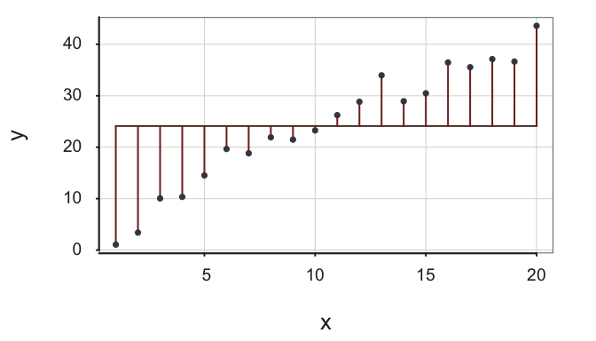
How well does the null model do in accounting for the variability of \(x\)? Continue to assess variation of \(y\) based on the usual sum of squared errors, SSE. However, in this situation the fit index is the standard deviation of the data, the square root of the sum of squared deviations about the mean. The usual standard deviation summarizes the scatter about the flat regression line for the null model, prediction only from the mean of target variable.
2.5.2.2 Definition
This null model is a worst-case prediction scenario, predicting with no value of \(x\).
The question for regression models is if we can improve model fit beyond the null model by adding additional information to our prediction equation.
The null model serves as a baseline by informing us the efficacy of prediction without one or more \(x\) variables. How much would fit increase if we could add one or more predictor variables to our model? How much better does the proposed model fit compared to the baseline fit from the null model? Answering this question provides a related, but distinct, evaluation metric from the scatter about the regression line given by \(s_e\).
The comparison of the scatter about the proposed regression model with \(x\) as a predictor and the null model with no \(x\), in terms of their corresponding sum of squared errors, results in another fit statistic.
The \(R^2\) fit statistic compares the residual variation of the proposed regression model with one or more \(x\) values to the size of the residual variation about the null model. \(R^2\) assesses the usefulness of the \(x\) features for predicting the value of the target \(y\) by comparing the fit of two different models. \(R^2\) compares the fit of the proposed model to the baseline model of not having the information provided by the features, the predictor variables. Without any statistical contribution, or even knowledge, of the \(x\) variables, how to predict the value of \(y\)?
The value of \(R^2\) varies from 0 to 1. A value of 0 indicates that the least-squares regression line of interest does not reduce the sum of the squared errors from the value obtained with the null model. \(R^2=0\) indicates that features X contribute nothing to the fit of the model. On the contrary, a value of \(R^2=1\) indicates a perfectly fitting model.
Figure 2.12 illustrates the two models, with the two different amounts of variability for the residuals, for the same data. The result is a relatively high value of \(R^2\). The scatter about the regression line of interest is considerably smaller than the corresponding scatter about the flat, null model line. Including \(x\) in the model to fit \(y\) provides a substantial improvement of fit compared to the model without \(x\).
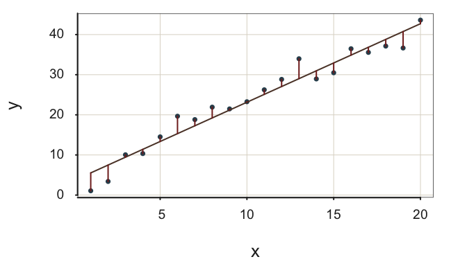

The regression line in Figure 2.12 fits the data well in two ways.
- The residuals about the regression line tend to be small, \(s_e=\) 2.71.
- The substantial reduction in the size of the residuals from the null regression model to the regression model with \(x\) indicate a value of \(R^2\) close to \(1\), \(R^2= 0.95\).
The example shown here illustrates the meaning of \(R^2\). Real data, however, typically does not reveal values of \(R^2\) this large.
Both fit indices in Figure 2.13 indicate fit more likely obtained with data: (a) Relatively large residuals about the regression line and (b) not so much reduction in variability from the null model to the regression model of interest.
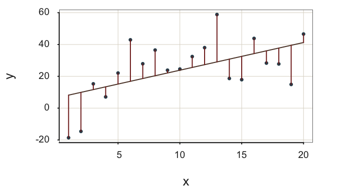
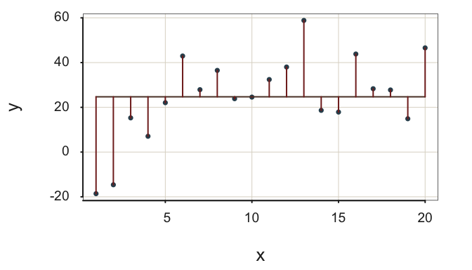
For this only moderately-well fitting model \(s_e=\) 16.24, and only a modest reduction in the size of the residuals from the null regression model to the regression model with \(x\), \(R^2=\) 0.30. In many applications, however, interpret an \(R^2\) of 0.30 or larger as a reasonably successful model, though the model can hopefully be refined for better fit, such as adjusting the functional form of the relation between each feature and the target, or by adding more features.
As shown next, compare the two sets of the sum of squares about the corresponding regression by their ratio.
2.5.2.3 Define
Express the amount of variability of the residuals as the corresponding sum of squares, \(\textrm{SSE} = \Sigma (y_i - \hat y_i)^2\), for each row of the data table. As indicated, the sum of squares for the proposed regression model with \(x\) applied to the data is SSE.
For the null model, deviations about the mean comprise the total sum of squares, SSY. This sum of squared deviations about the mean is the core of the definition of the standard deviation of \(y\), the square root of the average squared mean deviation. The sum of squared errors for the null model also appears in the ANOVA table shown in Figure 2.8. Here the associated sum of squared deviations is about the flat line, the mean, for the variable Weight.
\[SS_{Weight} = 7324.900\]
SSE and SSY respectively indicate the corresponding size of the squared residuals for the model of interest with \(x\) and the null model without \(x\).
Comparing SSE and SSY is comparing scatter about the fitted value for the model of interest, \(\hat y_i\), to the fitted value for the null model, \(m_y\) for all values of \(x\). Compare SSE to SSY as their ratio. Define \(R^2\) as the ratio of SSE to SSY, arbitrarily subtracted from 1 so that higher values indicate better fit.
\[R^2 = 1 - \frac{SSE}{SSY} = 1 - \frac{\Sigma (y_i - \hat y_i)^2}{\Sigma (y_i - m_y)^2}\] Squared deviations about the sloped regression line from \(x\) tend to be smaller than squared deviations about the flat regression line from the null model. How much smaller? In this example, squared deviations about the sloped regression line are about 60% of the squared deviations about the flat line, or 40% when subtracted from 100%.
\[R^2 = 1 - \frac{SSE}{SSY} = 1 - \frac{4386.674}{7324.900} = 0.401\]
2.5.2.4 Interpret
The value of \(R^2\) ranges from 0 to 1.
\(R^2\) indicates the proportion of variance of \(y\) accounted for by the proposed model. The lower extreme of 0 indicates no advantage to the proposed model in explaining values of \(y\). The upper extreme of 1 indicates a perfect fit, all variance of \(y\) is explained by the model.
No relation between features X and target \(y\) yields \(R^2=0\). In this situation, the features X contribute nothing to predictive efficiency. The proposed regression line with \(x\) in the model is as flat as the the null model line, \(\hat y_i = m_y\), so SSE = SSY.
\[R^2 = 1 - \dfrac{SSY}{SSY} = 1 - 1 = 0\]
For the best-case scenario, X perfectly relates to \(y\). In this case, the values calculated from the regression model exactly equal their corresponding data values. Perfect fit implies \(\hat y_i = y_i\), so SSE = 0.
\[R^2 = 1 - \dfrac{SSE}{SSY} = 1 - 0 = 1\]
As a general, but only approximate guideline not necessarily applicable to every situation, interpret \(R^2\) as follows.
- 1 indicates perfect fit
- 0.6 is usually considered excellent fit
- 0.3 is usually considered adequate fit
- 0 indicates the regression model provides no improvement over null model
All regression software provides the estimated value of \(R^2\), and, usually, related values. For the analysis of the toy data set example from Table Table 2.2, the lessR output follows.
R-squared: 0.511 Adjusted R-squared: 0.450 PRESS R-squared: 0.307☞ Evaluate fit with \(R^2\).
The \(R^2\) value of 0.511 is generally considered to provide a reasonable level of fit, a practical reduction in the size of the residuals of the given model compared to the null or flat-line model, though with considerable room for further improvement.
Unfortunately, \(R^2\) only describes fit to the particular training sample from which the model was estimated. As seen from this output, other versions of \(R^2\) also exist, which are more general than the original \(R^2\). In particular, PRESS \(R^2\), defined later, is not always provided by other software but included in the lessR regression analysis.
2.5.2.5 Compare
The two fit indices, \(s_e\) and \(R^2\), provide complementary information. The standard deviation of the residuals, \(s_e\), and its squared version, mean square error, MSE, indicate the amount of scatter, the size of the residuals, about the regression line. \(R^2\) alternatively compares the size of the model’s residuals to the residuals from the baseline null model in which no information is provided for variables other than \(y\) itself. However, \(R^2\) by itself does not indicate the amount of scatter about the line per se, but rather how much the scatter is reduced from the null model.
\(s_e\) is an absolute fit index, focused on the size of the residuals, whereas \(R^2\) is a relative fit index, which compares the size of the residuals from the proposed model to those of the null model.
As such, the two fit indices do not always provide the same indication of fit, such as shown in Figure 2.14.
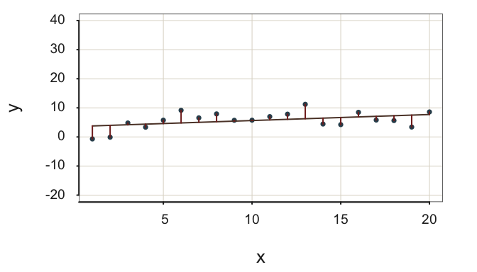
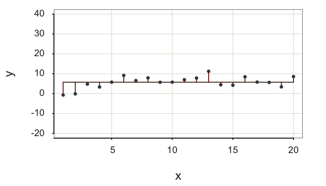
Figure 2.14 demonstrates little variability about an almost flat regression line. The residuals are small, their standard deviation is only \(s_e=\) 2.71, which indicates little scatter about the regression line in Figure 2.14, given the units in which \(y\) is expressed. However, there is also little variability in the target \(y\), so the null model does almost as well as accounting for the values of \(y\) as does the regression model with a non-zero \(b_1\), that is, the model of interest with \(x\). \(R^2\) in this situation of little variability in \(y\) indicates poor fit, with \(R^2=\) 0.18. As Figure 2.14 illustrates, the model of interest with non-zero \(b_1\) contributes little more to prediction efficiency than does the null model.
A small value of \(s_e\) does not imply worthwhile fit if \(R^2\) is also small.
Yes, a goal of model building is to attain a small sum of squared residuals, that is, little scatter about the regression surface, a line when plotted in two dimensions. Simultaneously, the target variable must exhibit variability, otherwise there is little to predict. In the extreme case in which all values of the target are the same, the prediction of the next value is simply that constant value. A prediction model adds value when the value of the target variable has a range of variability, yet the model accurately predicts the value of the target, particularly when evaluated on new, testing data.
2.5.3 Fitted vs Predicted
The model’s fit to the training data, the data from which the model is estimated, is only the starting point for evaluating model fit. The training data contains both the data values for the features, the predictor variables, and the target variable’s data values. There is no prediction with the training data because the target values are already known. We do not predict what we already know.
We have seen that the fitted value is the value of \(\hat y_i\) calculated from the prediction equation given a specific value of \(x\), \(x_i\). The value \(\hat y_i\) fits the model. However, the fitted value is a prediction only when the answer is not known in advance.
Of ultimate interest is the fit of the model to testing data, that is, new data for which the model has not been trained (estimated). The previous applications of \(MSE\) or \(s_e\) and \(R^2\) evaluate model fit to the training data, usually biased higher than when the model is generalized to new data. Understanding the level of fit to the training data is only a start to the process of model evaluation.
The true evaluation of the model considers how well the model fits new, previously unseen data and how well it predicts when the value of \(y\) is not known.
Unfortunately, fitting the training data well does not necessarily imply that the model will generalize to predicting the values of \(y\) from new, previously unseen data from which the model was estimated.
The fitted values being close to the actual value of \(y\) is a necessary condition for effective prediction but is not sufficient to guarantee predictive accuracy. The versions of the fit indices \(MSE\) or \(s_e\) and \(R^2\) when applied to new data generally show poorer fit than the model developed on the training data. If the model fits the training data well, and the new data almost as well, however, then the model may be ready to be deployed for actual prediction.