Usually we would plot the data before applying a forecasting algorithm. However, we have already done this. We know from before that the process is stable, that is, random fluctuations around the center.
Use the simple exponential smoothing function, ses(), from the forecast package to forecast the time series five quarters ahead. Save the output in the object fit. Because the output was directed to an object, for future reference, there is no output at the R console.
fit <-ses(Y3_ts, h=5)
Examine the model parameters, which for simple exponential smoothing, is \(\alpha\). The algorithm chooses the value of \(\alpha\) that minimizes the mean of the squared errors.
The smoothing algorithm chose an extremely low value, \(\alpha\) = 0.0001. The reason is that the process is stable, consisting of nothing more than random fluctuations about the same mean with a constant level of variation. With pure randomness, there is no gain from referencing forecasting error from the current time to adjust the forecast for the future time. All data values result from random fluctuation about the mean. Hence, \(\alpha \approx 0\).
Display the contents of the fit object to view the forecasts.
fit
        Point Forecast    Lo 80    Hi 80    Lo 95    Hi 95
2017 Q3       50.19771 49.29586 51.09955 48.81846 51.57696
2017 Q4       50.19771 49.29586 51.09955 48.81846 51.57696
2018 Q1       50.19771 49.29586 51.09955 48.81846 51.57696
2018 Q2       50.19771 49.29586 51.09955 48.81846 51.57696
2018 Q3       50.19771 49.29586 51.09955 48.81846 51.57696
Because the process is stable, each forecasted value is the same, a value very close to the mean of Y3, \(m\) = 50.189.
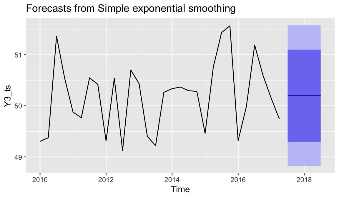
With the autoplot() function, plot the data and the forecasts, with the 80% and 95% prediction intervals.
autoplot(fit)
For this stable process the prediction intervals essentially span the range of the data. The forecast indicates properly indicates that the next value of the time series will likely lie within the specified range of data centered over the mean.
4.2 Forecast from Trend + Seasonality
With this example, begin with a time series characterized by both trend and seasonality, as seen from a previous homework.
d <-Read("http://web.pdx.edu/~gerbing/0Forecast/data/Sales07.xlsx")
[with the read.xlsx() function from Schauberger and Walker's openxlsx package]
Data Types
------------------------------------------------------------
character: Non-numeric data values
integer: Numeric data values, integers only
double: Numeric data values with decimal digits
------------------------------------------------------------

    Variable                  Missing  Unique
        Name     Type  Values  Values  Values   First and last values
------------------------------------------------------------------------------------------
 1      Year   integer     16       0       4   2016  2016  2016 ... 2019  2019  2019
 2       Qtr character     16       0       4   Winter  Spring ... Summer  Fall
 3     Sales    double     16       0      15   0.41  0.65  0.96 ... 2.11  2.25  1.74
------------------------------------------------------------------------------------------
Simple exponential smoothing does not account for trend and seasonality, and so does not apply to this time series. To illustrate the mismatch, apply this forecasting procedure to these data, again with the ses() function from the forecast package.
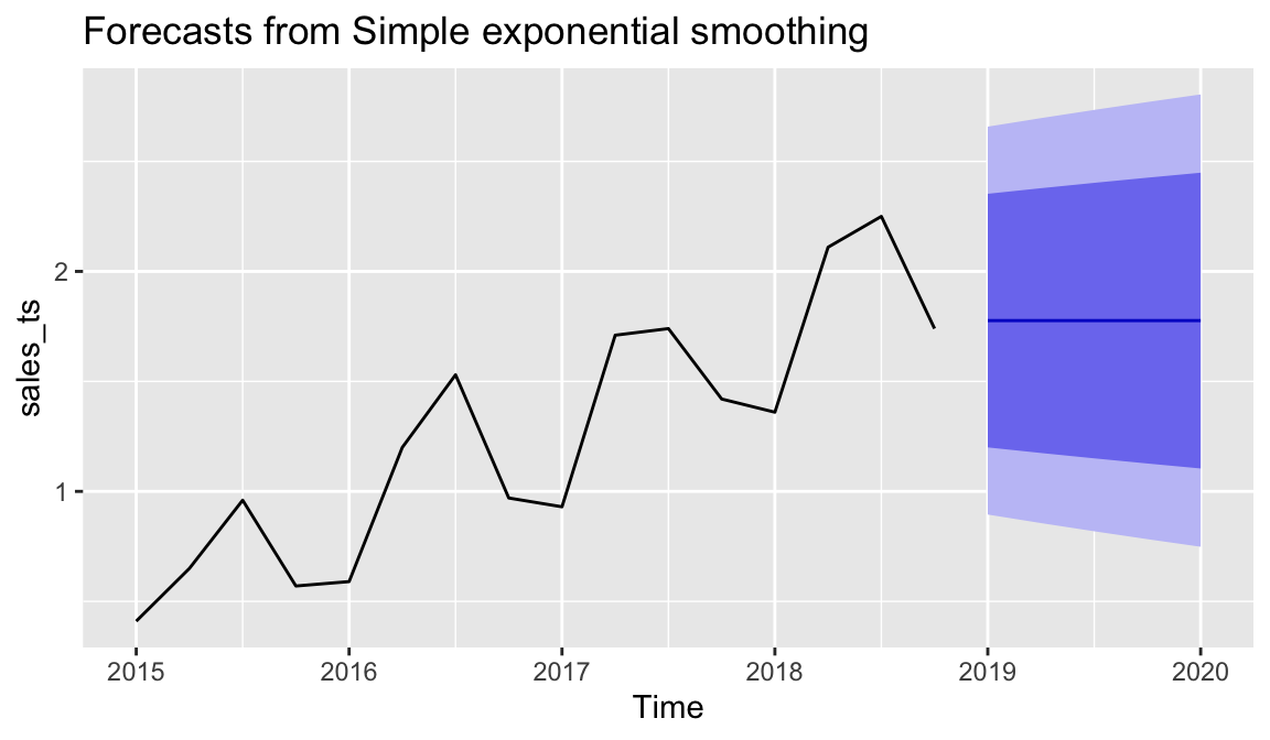
To illustrate the parameter alpha, first set \(\alpha=0.3\).
fit <-ses(sales_ts, alpha=.3, h=5) fit$model # model parameters
The reported value of sigma is the standard deviation of the residuals of the component of output called model that the ses() function created. Here, \(s_e=0.450\). Compare this value across models to better understand which model is functioning more effectively.
View the forecasted values and corresponding prediction intervals, and plot.
fit
        Point Forecast    Lo 80    Hi 80     Lo 95    Hi 95
2019 Q1         1.7764 1.199957 2.352842 0.8948068 2.657993
2019 Q2         1.7764 1.174576 2.378224 0.8559897 2.696810
2019 Q3         1.7764 1.150223 2.402577 0.8187447 2.734055
2019 Q4         1.7764 1.126782 2.426018 0.7828950 2.769905
2020 Q1         1.7764 1.104158 2.448642 0.7482946 2.804505
autoplot(fit) # visual forecast
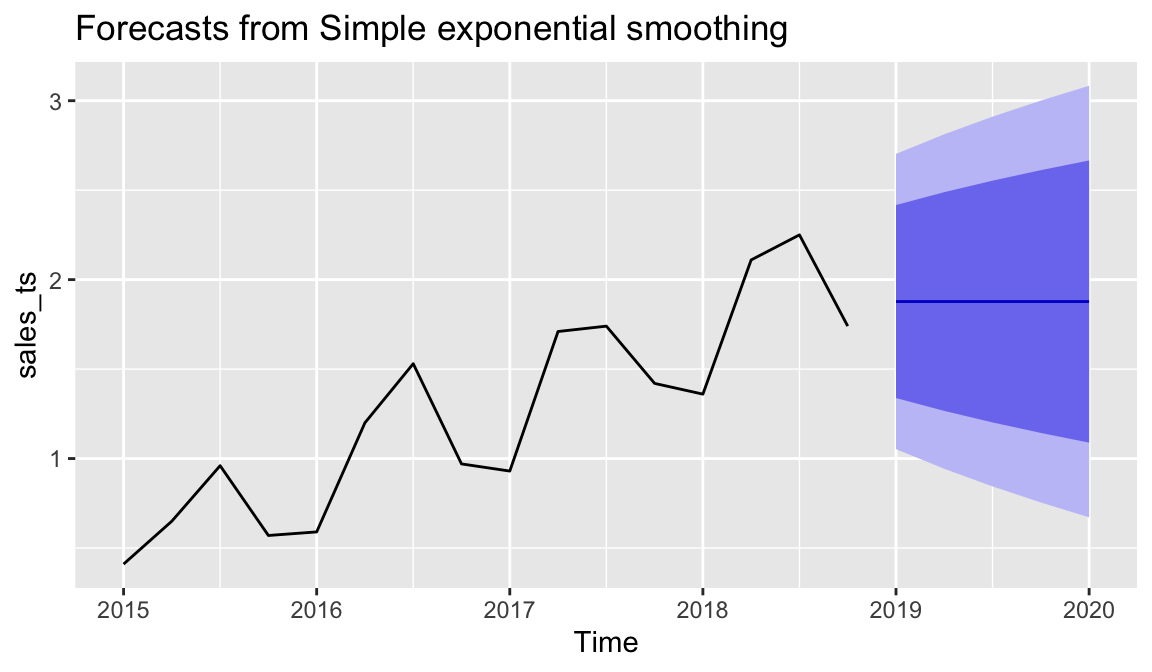
Here let ses() choose the value of \(\alpha\) that yields the best fit to the data.
fit <-ses(sales_ts, h=5)fit$model # model parameters
The smoothing algorithm chose \(\alpha\) = 0.5334.
View the forecasted values and corresponding prediction intervals, and plot.
fit # numeric forecast
        Point Forecast    Lo 80    Hi 80     Lo 95    Hi 95
2019 Q1       1.877535 1.338198 2.416871 1.0526910 2.702378
2019 Q2       1.877535 1.266279 2.488790 0.9426994 2.812370
2019 Q3       1.877535 1.201973 2.553096 0.8443518 2.910717
2019 Q4       1.877535 1.143277 2.611792 0.7545846 3.000484
2020 Q1       1.877535 1.088938 2.666131 0.6714805 3.083589
autoplot(fit) # visual forecast
Best fit of \(\alpha\) or not, clearly simple exponential smoothing does not properly apply to this time series with trend and seasonality. There is no trend or seasonality in the forecast for next year’s values.
4.4 Exponential Smoothing of Trend
The Holt adaptation of exponential smoothing adds a second parameter, \(\beta\), to account for underlying trend, but not seasonality. Illustrate with the holt() function from the forecast package. View the chosen model parameters.
The value of sigma, the standard deviation of the residuals, decreased from \(s_e=0.450\) for the SES analysis to \(s_e=0.320\) when accounting for linear trend.
fit # numeric forecast
        Point Forecast    Lo 80    Hi 80    Lo 95    Hi 95
2019 Q1       2.127147 1.717305 2.536989 1.500347 2.753947
2019 Q2       2.229319 1.819476 2.639161 1.602519 2.856119
2019 Q3       2.331490 1.921648 2.741333 1.704691 2.958290
2019 Q4       2.433662 2.023820 2.843504 1.806862 3.060462
2020 Q1       2.535834 2.125991 2.945676 1.909034 3.162634
autoplot(fit) # visual forecast
The Holt method forecast does account for the trend. However, the forecasts still are not optimal because the method does not account for underlying seasonality.
4.5 Exponential Smoothing Trend and Seasonality
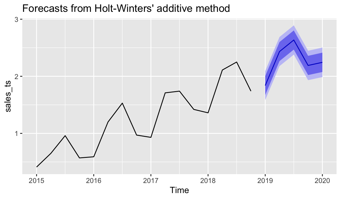
Holt-Winters, or triple exponential smoothing, is the preferred smoothing method for data characterized by both trend and seasonality. Use the hw() function from the forecast package.
The value of sigma, the standard deviation of the residuals, decreased from \(s_e=0.450\) for the SES analysis to \(s_e=0.320\) when accounting for linear trend. Accounting for trend and seasonality lowered the standard deviation to \(s_e=0.129\), a substantial and meaningful reduction.
Get the numeric forecasts, prediction intervals, and the visualization.
fit
        Point Forecast    Lo 80    Hi 80    Lo 95    Hi 95
2019 Q1       1.838427 1.672779 2.004074 1.585091 2.091762
2019 Q2       2.433648 2.267112 2.600184 2.178954 2.688342
2019 Q3       2.635763 2.468341 2.803185 2.379714 2.891813
2019 Q4       2.189985 2.021680 2.358291 1.932584 2.447387
2020 Q1       2.244745 2.075555 2.413935 1.985991 2.503498
autoplot(fit)
The hw function provides two seasonal methods, "additive" and "multiplicative". The default is "additive". To estimate a multiplicative model, set the parameter seasonal to "multiplicative".