3.1 Data Table
Data analysis begins with, well, data. Analyze the data values for at least one variable, such as the annual salaries of employees at a company. Organize the data values into a specific structure from which the analysis proceeds. To learn how to use a data analysis system such as Python, first understand the organization of data values into a data table [video 5:14].
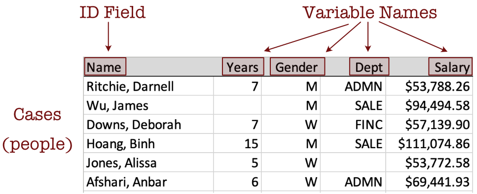
Data Table: A rectangular arrangement of data values, with the values for each variable in a column and the name of the variable at the top of the column.
Store the structured data values within a computer file, such as an Excel file or a text file. This file can be stored on your computer, an accessible local network, or the world wide web. The data table in Figure 3.1, formatted as an Excel file, contains four variables: Years, Gender, Dept, and Salary, plus an ID field called Name, for a total of five columns.
Describe the data table by its columns, rows, and cell entries.
Data value: The contents of a single cell of a data table, a specific measurement.
Variable name: A short, concise word or abbreviation that identifies a column of data values in a data table.
Example: Each row of the data table, the data for a specific instance of a single person, organization, place, event, or whatever is studied.
Unfortunately, data analysis terminology is not standardized. Other names for an example are data row, case, sample, and instance. Even more confusingly, in some contexts, the word sample refers to all the rows of data values, and in other contexts, it refers to a single row of data.
Figure 3.1 shows the data values in the Excel file for just the first six employees. For example, according to the data values for employee Darnell Ritchie, he has worked at the company for seven years, identifies as male, and works in administration, with an annual salary of $53,788.26. Two data values in this section of the data table are missing. The number of years James Wu has worked at the company is not recorded, nor is the department in which Alissa Jones works.
Encode the data table in one of several computer file formats. The formats we encounter are Excel files, indicated by a file type of .xlsx, and text files in the form of comma-separated value files, indicated by .csv. A text file can have one of several potential file types, such as .txt, but for data tables is usually .csv.
csv file: A data file that consists only of text, with adjacent data values for each row of data separated by commas.
The first five rows of the employee data file in csv format appear in Figure 3.2.
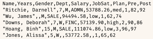
An advantage of csv files is that any computer app that reads text can read them. They are also the default text file type for Excel.
Data analysis can proceed only after the data table is identified and the relevant variables are identified by name.
All Python data analysis functions analyze the data values for one or more specified variables, identified by their names, such as Salary.
Analysis requires the exact spelling of each variable name, including the same pattern of capitalization.
3.2 Read Data
3.2.1 Data Frame
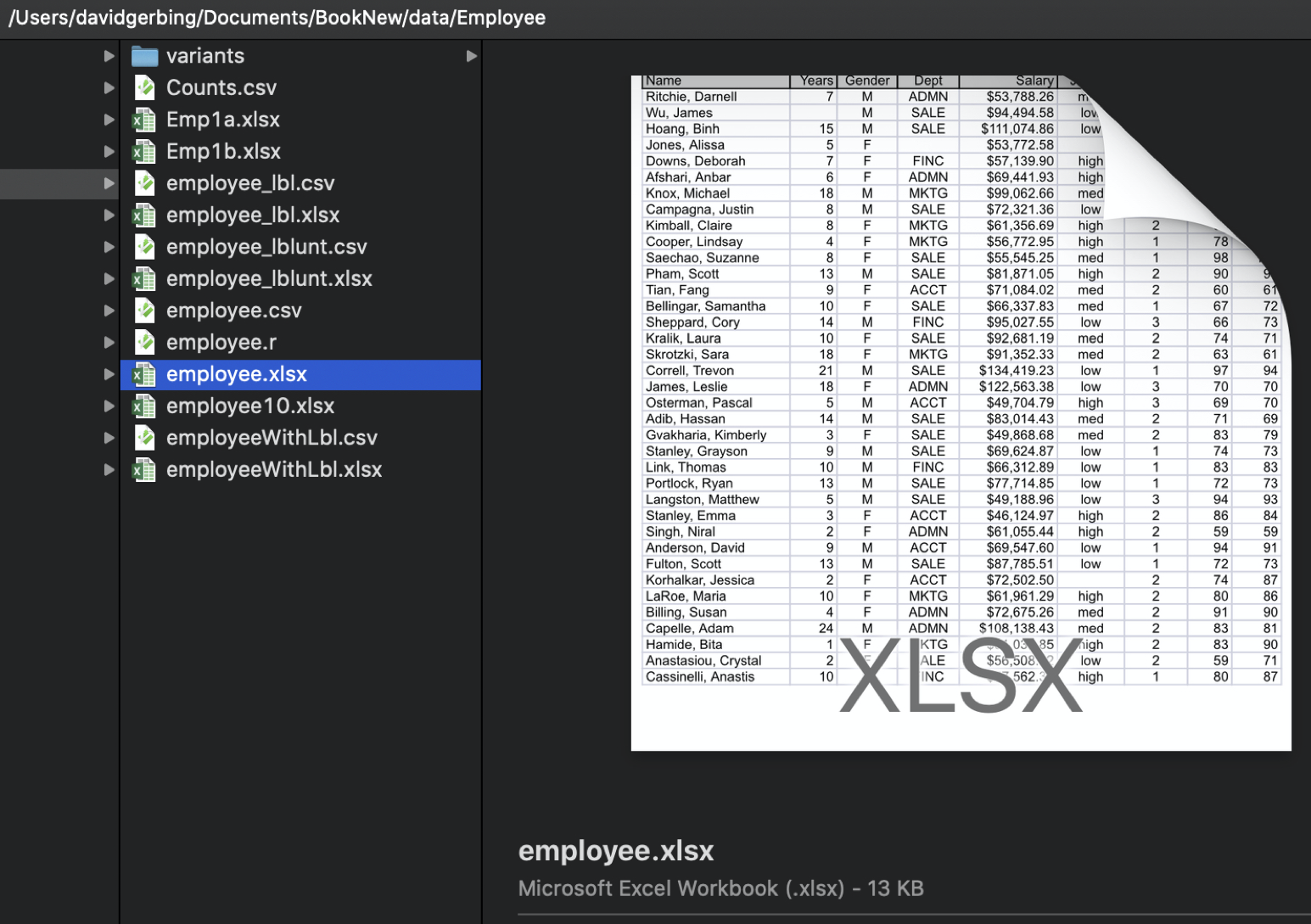
To begin an analysis, read the data from a computer file into Python. Your data organized as a data table exists somewhere as a data file stored on a computer system. Figure 3.3 shows a data table as an Excel file named Employee.xlsx stored on a (Macintosh) computer. Figure 3.1 shows the first several lines of this data table in detail.
The data table stored within a running Python program has its own name.
Data frame: A data table stored within a Python session as a pandas data structure.
Each variable in a data table has a name, and so does the data table itself. Reference the data table stored on your computer system by its file name and location. When reading the data table into Python, assign the resulting data frame a name of your choice. Regardless of the file name on your computer system, typically name the data table within the active Python session, the data frame, simply d for data.
When analyzing data read into Python, the same data exists in two different locations: as a computer file on some computer system, and as a Python data frame within a running Python app. Different locations, different names: same data. On your computer system, identify the data table by its file name and location. Within a running Python app, identify the same data by its data frame name.
To read data from a file into a data frame of a running Python application, as with every other task in Python, invoke a function. The pandas package provides two functions for reading data into a pandas data frame.
read_csv(): Read a data table in a file formatted as csv text, with adjacent data values separated by commas.
read_excel(): Read a data table in a file formatted as an Excel file.
Specify the location of the data file within quotes as the first value passed to each function, within the parentheses. Specify either the path name of a file on your computer system or a web address that locates the data table on the web. Chapter 8, Read Data, of the video illustrates reading data into the d data frame.
Because the read functions are from the pandas package, inform Python of this location by beginning each function call with pd.
d = pd.read_csv("path name" or "web address")d = pd.read_excel("path name" or "web address")With Excel, Python, and other computer apps that process data, enclose character strings, such as file names, in quotes. For example, to read the data stored on the web in the data file called employee.xlsx into the data frame d, invoke the following function call.
Because Python organizes analyses by variable name, it is crucial to know the exact variable names, including the pattern of capitalization.
Specify a Python analysis for one or more variables, the columns in the data frame.
Rows and columns organize a data table. The variables are in the columns, so to specify a variable is to specify a column of data values.
3.2.2 From the Web
Figure 3.4 illustrates reading the data from an Excel file employee.xlsx on the web.

If using Jupyter Lab as the development environment, enter the function call to read the data into a notebook cell.
3.2.3 From Colab
Access Colab at colab.research.google.com. Colab uses your Google Drive for file storage. When you open a Colab notebook stored on Google Drive, the notebook itself is available immediately. However, any data files stored on Google Drive are not automatically available to the Python runtime.
If you have a data file to read that is not on the web, create a data folder on your Google Drive and move the data file to that location. To access your Google Drive on the web, go to drive.google.com. Better, however, download the Google Drive app to your device for direct local access.
To read a data file from Google Drive into Colab, first import the drive module from google.colab. Then mount Google Drive into the active Colab session with the drive.mount() function. Mount the drive directory, or folder, in the content directory as follows. When you request to mount the drive, Colab asks for authorization to access your Google Drive files.
from google.colab import drive
drive.mount('/content/drive')
After mounting the drive, reference files on Google Drive with the folder path /content/drive/MyDrive/. For example, if the file employee.xlsx is stored in a Google Drive folder named data, read the file into the data frame d as follows.
d = pd.read_excel('/content/drive/MyDrive/data/employee.xlsx') The full file reference also contains the string MyDrive, which accesses your Google Drive. This example presumes that you created a folder on your Google Drive called data that contains your data files.
Note the path name is included within quotes.
3.3 Display Data
r newthought(“To analyze data, you need to understand the data.”) You should know what the data values look like for each variable, and you should know the variable names. After reading the data into Python, view the contents of the newly created data frame. To view the contents of any Python object, enter the name of the object. Here, enter the name d to view all the data.
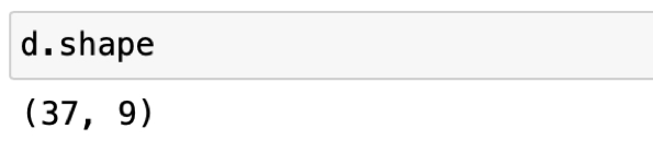
Of course, viewing all the data is usually not practical. Instead, display [video 4:28] part of the data, including the size of the data table. The shape attribute shows the number of rows and then columns in the data table. The output appears in Figure 3.5.
Or, use the head() function to list the variable names and, by default, just the first five rows of data, here for the data frame d. Figure 3.6 illustrates the head() function.
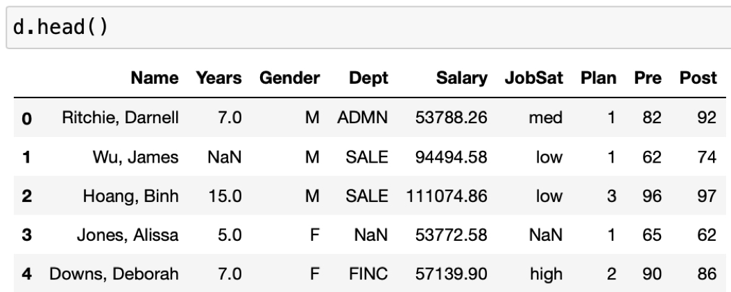
The following output from the Python data frame d results.
Compare this output, the representation of the data within Python, to the data table in Figure 3.1 as an Excel file. Same data, different locations. Note the pandas representation of missing data.
Python missing data code:
NaNfor not a number.
The blank cells in the Excel file, Figure @ref(fig:dataTable), are replaced with either NaN.
Python pandas also provides a corresponding function tail() that lists the data values at the end of the file.
3.4 Two Types of Variables
Always distinguish continuous variables from categorical variables. This distinction between the two types of variables is fundamental in data analysis.
Continuous (quantitative) variable: A numerical variable with many possible values.
Categorical (qualitative) variable: A variable with relatively few unique labels as data values.
Examples of continuous variables are Salary and Time, both defined on a numerical scale with many unique values. Examples of categorical variables are Gender and State of Residence. Each categorical variable has relatively few possible values compared to a continuous variable. The distinction between continuous and categorical variables is common to virtually every data analysis project.
Sometimes the distinction becomes confusing because variables with integer values, which are numeric, can be quantitative or qualitative. For example, Man, Woman, and Other could be encoded as 0, 1, and 2, respectively, for three levels of the categorical variable Gender. However, these integer values are just labels for different non-numeric categories. Best to avoid this confusion. Instead, encode categorical variables with non-numeric values. For example, encode Gender with M, W, and O for Other.
To distinguish between continuous and categorical variables, determine if the values of a variable are on a numerical scale, presumably with a relatively large number of unique values that can be ordered from smallest to largest. A categorical variable such as Gender, however, remains categorical even when coded numerically. For example, Woman coded as 1 is not more than Man coded as 0, or vice versa.
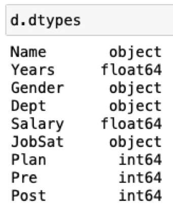
Python, like all computer applications, stores numerical and categorical data differently. After reading the data into a data frame, pandas provides an attribute to show the storage type of the data values for each variable.
dtypes: Attribute to display the name of each variable in the specified data frame and its associated data type.
When calling the attribute, precede it with the data frame name and a period.
The Python variable types we work with follow.
- categorical variables: object or category
- integers: int64
- numbers with decimal digits: float64
Figure 3.7 illustrates the input and output of dtypes.
The distinction between the variable types object and category is discussed later. For now, object is the default variable type for a non-numeric variable. Eventually, however, all categorical variables, whether integer-coded or character strings, should be converted to the variable type category. First, memory is better conserved, and second, meaning is better communicated.