2 Jupyter Notebook

Jupyter Notebook is a standard document format for developing and running Python programs.

Jupyter Notebook: A free, open-source web application for creating and sharing interactive documents that contain Python code, output, and explanatory text.

Many environments are available for developing and running Python code. Jupyter Notebook is one of the most widely used formats for beginning data analysis because it combines code, results, and explanatory text in one document.

To run our first Python program, we need to understand two concepts at the same time:

• Jupyter Notebook: How to enter and run Python code, view results, and add explanatory text.
• Python: The syntax of a Python function call.

We need to know something about the development environment, and we need to know enough Python to enter and run at least one specific function call. We begin with a description of Jupyter Notebook.

2.1 Access a Notebook

To begin or continue a Python analysis, open a new or existing Jupyter Notebook, which opens in your default web browser. Identify Jupyter Notebook files by their filetype of .ipynb for Interactive PYthon NoteBook. As with most files in modern data analytics, including machine learning, .ipynb files are non-proprietary standard text files that a standard text editor could edit outside the development environment. However, a Jupyter Notebook renders the structure of the text file in convenient notebook form and provides the run time environment for executing Python code.

2.1.1 Miniconda on Your Computer

Before opening a notebook, first create a folder to store all notebooks and data files. A suggestion is a folder called Python in your Documents folder, and then a folder called Data within the Python folder.

To access the notebooks, begin by entering the Jupyter Notebook environment. Specify the base installation of Miniconda, then launch Jupyter Notebook from the command line:

conda activate base
jupyter notebook

Jupyter Notebook opens in the directory from which it is launched. The resulting Jupyter browser window shows the contents of that directory. From there, navigate to the folder that contains your course notebook files.

• Create a new notebook: From the Jupyter file browser, click the New button in the top-right corner and then choose a menu item such as Python 3 to create a new notebook.
• Open an existing notebook: From the Jupyter file browser, click the .ipynb notebook file
• Save an existing notebook: Click the disk icon or File --> Save in the Jupyter Notebook file menu (not the browser menu)
• Close the notebook: Select File -> Close and Shut Down Notebook
• Stop Jupyter Notebook completely: Return to the Terminal or Anaconda Prompt window where Jupyter is running. Press Control-C. If prompted, type y and press Enter.

2.1.2 Colab in the Cloud

Enter Google Colab through a browser linked to Colab at colab.research.google.com. Once there, bookmark the site for an easy return. Colab will automatically create a folder on your Google Drive called Colab Notebooks in your MyDrive folder, and then store your Python Notebooks in that folder. A suggestion is to create your own data folder at the top level of MyDrive to store your data files.

To open a Notebook: Go to the File menu and select New notebook. Change the notebook name by clicking on the name at the top of the window. Another way to open a Colab Notebook is directly from Google Drive. Locate the notebook in the Colab Notebooks folder, right-click, choose Open with, then Google Colaboratory.

2.2 Do Python

Now we have the information we need to start building a Python program.

2.2.1 Cells

A notebook, such as Jupyter Notebook, is a computer document that consists of an ordered collection of cells, one after the other. To enter information into a Jupyter Notebook is to enter information into a specific cell. A cell contains one of two types of information.

Cell: A self-contained block of code or narrative text.

Work with the information in a cell separately from the information in other cells. The default type of cell is for code.

Code cell: Cell that contains code, such as Python code.

The purpose of the code cell is to enter and process Python code.

2.2.1.1 Jupyter Notebook

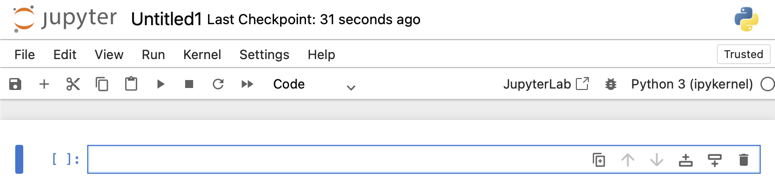
The new Jupyter Notebook file appears as a single blank cell with the name of Untitled.ipynb, shown in Figure 2.1.

Figure 2.1: New Jupyter Notebook notebook file that opens with a single code cell.

To interact with AI to fix errors, the nonworking code into an AI large language model such as ChatGPT and request a fix.

2.2.1.2 Colab

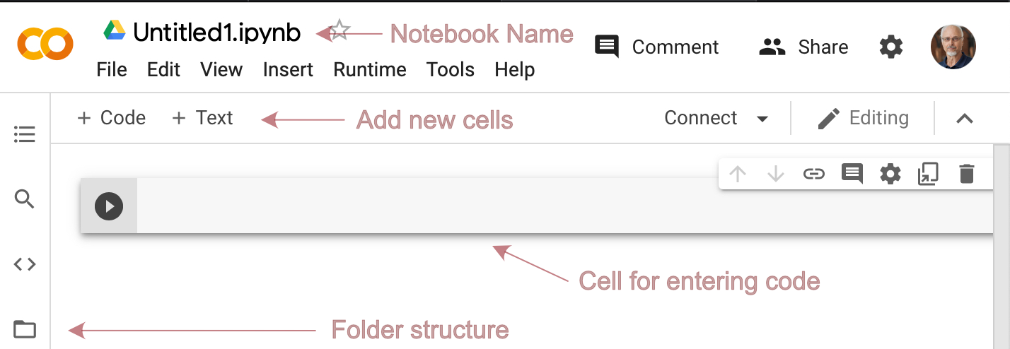
The Colab interface shown in Figure 2.2 is a little different from the standard Jupyter Notebook interface, but the concept is the same. To create a new notebook, go to the Colab menu, not the browser menu, and select:
File -> New notebook in Drive.

Figure 2.2: Create a new Python 3 Jupyter Notebook in Colab.

The generate link within a code cell calls Google’s Gemini AI. You can use Gemini to request Python code for common tasks, such as reading data into the notebook, creating a visualization, or running a complete machine learning analysis. If you enter an invalid Python instruction, Colab displays the standard Python error message.

Gemini can also provide an enhanced explanation of the error and suggest a correction. When Gemini suggests a correction, it may show the proposed change as a comparison. Lines marked with a minus sign and a red background are lines to remove. Lines marked with a plus sign and a green background are lines to add. At the end of the Gemini message, choose Accept to apply the correction, Accept & Run to apply and run it, or Cancel to reject it.

2.2.2 Edit and Command Modes

Working with a notebook cell involves two different activities. First, enter or edit the contents of the cell. Second, run the cell so that Python processes the code and displays the output. These two activities correspond to two notebook modes.

Edit mode: The mode for entering and editing the contents of a cell.

In edit mode, the cell works like a text editor. Enter the information, either Python code or explanatory text, directly into the cell.

Edit mode is indicated by:

• Jupyter Notebook: A colored border around the active cell.
• Colab: The active cursor inside the cell.

To enter edit mode, press Enter/Return, or double-click inside the cell.

Command mode: The mode for working with the cell as a notebook object rather than editing its contents.

Command mode is used to select, move, copy, delete, or run cells. To leave edit mode and return to command mode, press Esc.

Command mode is indicated by:

• Jupyter Notebook: A blue left margin or border on the active cell.
• Colab: The current cell available for action through controls such as the run arrow in the left margin of a code cell. Otherwise, there is no indication.

Running a code cell is a separate action. When a code cell is run, Python processes the code in that cell and displays any output below the cell. In both Jupyter Notebook and Colab, press Control/Command + Enter to run the current cell.

This runs the current cell and leaves the selection on that cell.

2.2.3 First Python Program

If the information entered into a code cell is a Python instruction, then that instruction can be run. According to tradition, the first instruction used when learning a new computer language displays the phrase Hello World.

Enter a line of Python code, as shown in these Hello World videos:

• Jupyter Notebook: First Time [2:17].
• Colab: First Time [2:52].

The process of running Python code involves entering one or more function calls, running the cell, fixing any errors, and then running the cell again. AI can often help explain error messages and suggest corrections, but the analyst still needs to review the suggested fix.

print() function: Display information as output.

The first Python function call, printing a single character string:

print("Hello World")

The quotes and parentheses are required. With Python, Excel, and other computer languages, character strings are enclosed in quotes. The print() function also requires the information to be displayed to appear inside parentheses. If the quotes or parentheses are omitted, Python generates a syntax error. Return to edit mode, fix the error, and then run the cell again.

Using the print() function provides the most control over displayed output. Jupyter Notebook and Colab also automatically display the result of the last line of a code cell when that line produces displayable output. This convention avoids the need for some print() statements, but the function remains useful when you want explicit or customized output.

A notebook almost always consists of more than one cell. Adding new cells is easy.

• Jupyter Notebook: From the Insert menu, either choose Insert Cell Above or Insert Cell Below. Newly created cells are initially Code cells. To convert a code cell to Markdown, choose the corresponding option from the menu at the top of the notebook window initially labeled Code.
• Colab: Clck the + Code or + Text button near the top of the screen. These buttons also appear when hovering with the mouse at the beginning or end of a cell.

In either environment, when not editing a cell, you can also press a to add a cell above the current cell, or b to add a cell below the current cell.

2.2.4 Markdown Text

2.2.4.1 Definition

A notebook can, and almost always should, contain narrative text that explains and describes the Python code and the resulting output. The finished notebook reads like a book chapter or a scrolling PowerPoint presentation, with explanation interspersed with Python code and output. Accordingly, there are two primary types of cells in a notebook.

Markdown text: A lightweight markdown language for creating readable, formatted text with a plain-text editor that uses embedded codes, such as for italics and headers, that format the text when the cell is rendered.

Enter the formatted text into a markdown/text cell.

Markdown cell (Jupyter Notebook) or Text cell (Colab): Cell for the display and formatting of narrative text.

Begin editing a markdown cell by pressing Enter/Return with the cursor over the cell, or by double-clicking the cell. A markdown cell can be rendered or unrendered. When rendered, the cell’s contents are displayed according to the embedded formatting. When unrendered, the text source of the cell is displayed for editing. In Colab, the editable, unrendered version and the rendered version are displayed simultaneously. To render the contents of a markdown/text cell, run the cell as if it were a code cell.

2.2.4.2 Bold and Italics

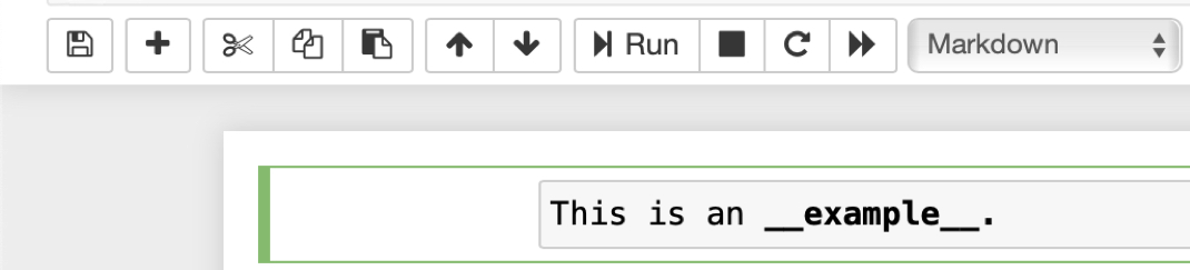
A variety of standard markdown codes apply across many environments, including Jupyter Notebooks. Markdown renders formatted text, such as text displayed on a web page, without requiring programming beyond the embedded formatting codes. Useful markdown codes include italics and bold. Italicize a word or phrase by beginning and ending it with either an underscore or an asterisk. Bold a word or phrase with two underscores or two asterisks. Rendering the corresponding text then displays the text according to these markdown instructions.

Figure 2.3 illustrates the unrendered version, the raw text, in Edit mode.

Figure 2.3: Markdown cell in edit mode.

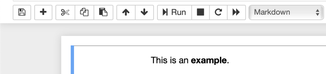
Render the text with Run or the corresponding icon from the window menu or with CMD/Return on a Mac. Find the rendered version in Figure 2.4.

Figure 2.4: Processed markdown cell to show formatting.

2.2.4.3 Headers

Another set of markdown codes formats a markdown cell as a header, useful for organizing the notebook into meaningful sections. Begin a line with a single pound sign, #, for a first-level header. A line that begins with two pound signs, ##, formats as a second-level header, and so forth.

2.2.4.4 Web Links

To create an HTML link, put the link text within square brackets, [ ] and then, immediately after, the URL in parentheses, (http://...).

2.2.5 Exit and Return

When your work in a Jupyter Notebook is complete for the moment, save your work and then exit then exit the system.

First, save your notebook:

• Jupyter Notebook: Click the disk icon at the top of the notebook window, or select File -> Save Notebook.
• Colab: Select File -> Save, or press Command/Control + S. Colab also saves automatically, but saving manually is a good habit.

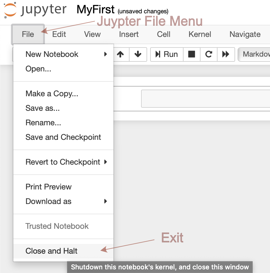
To close one notebook in Jupyter Notebook, select File -> Close and Shut Down Notebook. See Figure Figure 2.5.

Figure 2.5: Exiting a Jupyter Notebook on your computer.

When Jupyter Notebook runs on your computer, it starts background processes that continue running until you shut them down. Exiting a notebook involves more than closing the browser tab.

End the entire session:

• Jupyter Notebook: From the Jupyter file browser window, do the menu sequencie File -> Shut Down.
• Colab: Save the notebook and then close the browser tab or window. Because Colab runs in the cloud, there is no local Jupyter process to stop on your computer.

2.2.6 Re-Initialize a Notebook

When you later go back to work and reopen the notebook, all of your previous output is still displayed. The problem is that this output is only a display. The underlying variables and objects, such as the data frame that contains your data, are no longer active. They are just displayed text and images.

Re-initialize the notebook and restore all variables and objects, run the entire notebook:

• Jupyter Notebook: Click the double-arrow button at the top of the notebook window, which restarts the process from the beginning and runs all the cells.
• Colab: Go to the Runtime menu and choose Run all.

Then the notebook is restored to the same state it was in when the notebook was closed. All displayed output is now live, with the corresponding computed data values active.