Lecture 19
Multiple
Regression
A Few More Comments
on Simple Regression
Just a couple
of quick additional words on simple regression. A regression equation, such as
the following,
![]()
refers to the
regression line for the predicted values of y. The predicted values, ![]() , all fall
exactly on the line, because that is what we expect based on what we know about
x (at least it is our best guess). We can also write a regression equation
slightly differently:
, all fall
exactly on the line, because that is what we expect based on what we know about
x (at least it is our best guess). We can also write a regression equation
slightly differently:
![]()
Notice that, in
this equation, we refer to the actual obtained scores on the Y variable, the
y's. Unless we have perfect prediction, many of the y values will fall off of
the line. The added e in the equation refers to this fact. Simply put, the
above equation states that the actual values can be determined if we know the
y-intercept, the slope and the x values, plus some additional error. It would
be incorrect to write the equation without the e, because it would suggest that
the y scores are completely accounted for by just knowing the slope, x values,
and the intercept. Almost always, that is not true. There is some error in
prediction, so we need to add an e for error variation into the equation. The
actual values of y can be accounted for by the regression line equation
(y=a+bx) plus some degree of error in our prediction (the e's). Each of the
little vertical lines in the figure below refer to the e's, which are also
called residuals.
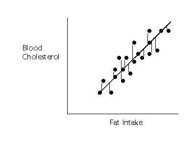
Another comment is
on notation. Often the regression equation is written in terms of the
population values, so the following equation is the regression equation for the
population values:
![]()
where b refers to the slope in the population. When
we refer to a particular sample with particular known slopes, intercepts, etc.,
we use the sample equation with the predicted scores on the left:
![]()
So in computer
output, you will rarely see residuals mentioned when the slope and intercept
are printed.
Multiple Prediction
Regression
analysis is a very general and useful tool. It also allows us to use more than
one independent variable to predict values of y. Take the fat intake and blood
cholesterol level study as an example. If we want to predict cholesterol as
accurately as possible, we need to know more about diet than just how much fat
intake there is. On the island of Crete, they consume a lot of olive oil, so
there fat intake is high. This, however, seems to have no dramatic affect on
cholesterol (at least the bad cholesterol, the LDLs). They also consume very
little cholesterol in their diet, which consists more of fish than high
cholesterol foods like cheese and beef (hopefully this won't be considered
libelous in Texas). So, to improve our prediction of blood cholesterol levels,
it would be helpful to add another predictor, dietary cholesterol.
Take a look at the
following diagram which illustrates who we can account for additional variation
of the Y variable by including another predictor:
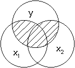
In this diagram,
the two predictors, x1 and x2, cover a larger area of the circle y. In the same
way, when there are two predictors of y, more of y's variation can be accounted
for. We have better prediction. If we add dietary cholesterol intake to fat
intake, we can better predict cholesterol levels.
From Two to Three
Dimensions
To represent this another way, geometrically, we now need to extend our
bivariate plot to a three dimensional one. With simple regression (one
predictor) we had only the x-axis and the y-axis. Now we need an axis for x1,
x2, and y. The plot of the data points is a three dimensional scatter plot,
with a swarm of points in a three-dimensional space. If we want to predict
these points, we now need a regression plane rather than just a
regression line. That looks something like this:
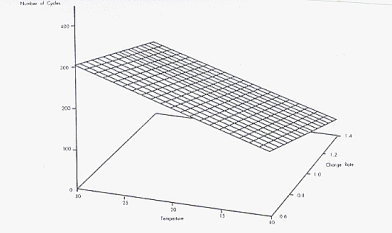
Multiple R2
Now we can think about how the two predictors together are associated with the
y variable. R-square is the amount of shared variation of the predictors with
y.
As before, we can
compute a sum of squares for the regression component, the error component, and
the total variation of y. The proportion of the total variation y (SST)
accounted for by x1 and x2 together (SSR) is equal to the amount of shared
variance (R2). Instead of a lower case r, as we used with simple
correlation, we now use a capital R, because we are estimating how much
variation x1 and x2, taken together, share with y.
R-square can be
understood several different ways. One way is to think in terms of the Venn
diagram, where the shaded area in the overlapping circles, represents the
amount of shared variance between x1, x2, and y. Another way to think about
R-square is the degree to which the points tend to fall off of the regression
plane. If the points all fall exactly on the regression plane, we have perfect
prediction. The x1 and x2 predictors account for 100% of the variation of the
criterion variable y. In this case, R-square is equal to 1.0. Most often, we
cannot predict y so perfectly, and many of the points will fall off of the
regression plane. How closely they swarm around the plane, however, indicates
how well our regression plane predicts the y scores. If the points form a long
semi-flat, oval shape (i.e., ellipsoid), there is a strong relationship. If
they are very dispersed in a round ball or cubic shape there is little or no
relationship.
"Partial"
Relationships
In the two predictor situation, we can still compute the correlation between
either of the predictors and the y variable. When we do this, we look at the
overall relationship of x2, for instance, and y. This is computed in the usual
way, and represents the standard correlation between x2 and y (sometimes called
the "zero-order" correlation). No information about x2 is used,
however. We can represent the correlation between x2 and y in the diagram
below.
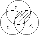
However, a useful
piece of information to know is how much one predictor overlaps with y
independently. That is, we want to know how much more information x2 provides
about y, over and above what we already know about x1. A depiction appears
below in the next figure:
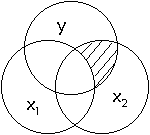
This is the
"partial" relationship between x2 and y. In our cholesterol example,
the partial relationship of x2 tells us how much dietary cholesterol predicts
blood cholesterol over and above the prediction from fat intake. There are
usually several ways researchers describe this type of partial relationship. We
might say that the partial relationship between x2 and y represents the
"independent contribution of dietary cholesterol to blood cholesterol levels,"
"the effect of dietary cholesterol on blood cholesterol after the effect
of fat intake is accounted for," "the effect of dietary cholesterol,
controlling for the effect of fat intake," or "the effect of dietary
cholesterol, holding constant the effect of fat intake." These are all
different ways of expressing the same thing.
Multiple Regression
Equation
The regression
equation can now be written as:
![]()
or
![]()
in which b1
(or b1) and b2 (or b2) represent the slopes for
the x1 or the x2 variable depending on whether we are speaking about the slopes
in the sample or the population.
The slope
coefficients now represent the independent or unique prediction of y for that
variable. They represent "partial" slopes so to speak. The prediction
of each independent variable is independent of the prediction of the other
independent variable.
An implication of
the partial slope is that the standardized version no longer represents the
correlation between x and y, because the slope represents a partial
relationship.
F-test and t-test
Just as before, we
have an overall test of the amount of variation in y that we can account for by
the predictors. For this, we are essentially testing the amount of shared
variation, the R-square, and how effectively we can predict the y scores
overall. The following table summarizes the F-test.
|
Source of Variance |
Sum of Squares Abbreviation |
SS Formula |
Interpretation |
Mean Square |
F-test |
|
Regression |
SSR |
|
Variation in the y variable explained by the regression equation. Deviation of the predicted scores from the mean. Improvement in predicting y from just using the mean of y. |
|
|
|
Residuals (or error) |
SSE |
|
Variation in the y variable not explained by the regression equation. Deviation of y scores from the predicted y scores. Error variation. |
|
|
|
Total |
SST |
|
Total variation in y. Deviation of y scores from the mean of y. |
not used |
|
In the above table,
k represents the number of predictors. In the examples up to this point, k=2.
With multiple
regression, the specific computations become too complicated to deal with, but
you should be aware of what each component of the analysis represents and what
the test means.
As with simple
regression, we can also conduct a t-test of the slope coefficients. In the
multiple regression context, there is more benefit to this test, because each
slope represents the partial relationship of its predictor to the dependent
variable. With simple regression, testing the slope with the t-test was
equivalent to testing the overall prediction equation, because there was only
one predictor available (remember that the standardized slope is equal to the
correlation in simple regression). Moreover, with multiple regression the
overall test of r-square can be significant, while not all of the slope
coefficients must be significant. One can think of the F-test as an omnibus
test that tests the regression equation in general.
More Than Two
Predictors
Multiple regression can also use more than two predictors. There is really no
limit to the number of predictors that can be included. At the very least, you
must have more subjects than predictors. Usually, people recommend that there
be 5 or 10 cases per predictor to have sufficient power. This is a very general
rule, because, as we know, power depends on many things. A careful power
analysis (which I won't cover in this class) is needed to truly determine the
sufficient sample size.
With more than two
predictors, the regression plane becomes a regression cube. Geometrically
speaking, instead of three dimensions, there would be four or five dimensions,
depending on how many predictors there are.
The general
(population) equation is usually written with an ellipsis to indicate that
there are other possible predictors in the equation:
![]()
where bk represents the last slope
and xk represents the last predictor variable. k represents the
number of predictors.


