suppressMessages(library(lessR))Introduction
Definition
Data in the real world typically does not arrive ready for analysis. On the contrary, most data analysts spend up to 85% their time preparing data for analysis. Instead, usually manipulate the data in various ways to derive a properly organized, clean, tidy data frame of rows by columns with all the data values in a column of the same type, such as character strings, integers, or floating-point numbers (i.e., with decimal digits).
Larger organizations have added a new job category called data engineer, a specialist in data wrangling and other aspects of handling data, beginning with data collection and organizing the entire flow through analysis, called the data pipeline.
Two Dialects
Before showing data wrangling in R and Python, first a discussion of what aspects of these languages are not covered.
R
The R ecosystem is bifurcated into two camps: Base R, downloaded from the R servers, and the Tidyverse, which is at least as popular as the corresponding Base R functions. Base R contains the essential packages and associated functions when R is downloaded, though there is some lacking functionality such as the inability to read Excel data files. My lessR package is designed to be consistent with Base R but simplify some of its syntax. The R functions presented in this document for data wrangling are primarily Base R functions with some lessR functions.
The Tidyverse comprises a series of packages developed by people associated with RStudio, now the Posit company. Most of these functions accomplish the same tasks as the corresponding Base R functions, albeit with much better marketing and organization. For example, the documentation for the tidyverse package of functions for data manipulation, dplyr, begins with a brief description of the five main verbs for data manipulations, the concepts of which form the material for this week. Listing all the related functions together and then calling the functions “verbs” for data manipulation is helpful. Although the base R documentation is not nearly so organized, all the functionality is there. Many Tidyverse users apparently do not understand that many of the same Tidyverse functions duplicate what has already been done, and that they favor the Tidyverse dialect because of better marketing, not better substance.
The situation is well summarized by an influential contributor to the R ecosystem.
R is rapidly devolving into two mutually unintelligible dialects, ordinary R and the Tidyverse.
He wrote a lengthy article on this issue. [Not required reading, reference should you be interested.]
This course covers both R and Python, with no room for also covering the Tidyverse dialect of R. The Tidyverse functions that would be covered here offer no functionality beyond the R and lessR functions already presented. Do be aware, however, that if you use the R language working with others, you may encounter Tidyverse enthusiasts who believe in its superiority. There is nothing wrong with the Tidyverse, per se, and if R were just beginning, I would have no problem if the R people adopted their functions in place of the Base R functions that have been adopted. However, in my opinion, given that we already have the Base R functions, we do not need the Tidyverse functions, and their presence creates confusion with a subtle commercial nudge toward Posit products.
Python
The Python language underwent a massive revision in 2008 when Python 3.0 was released. Although many improvements in the language were adopted, Python 3 was not backward compatible with Python 2. Many existing Python programs broke in the upgrade, so Python 2 remained in place simultaneously with Python 3. The result was about ten or so years of transitioning to Python 3. Today, that transition is largely complete and the confusion that resulted from the changes has mostly ceased with an improved language the result. Accordingly, this document focuses on Python 3.
Get Started
The following examples demonstrate useful data manipulations that apply to all data analysis: subsetting a data table, converting variable types, and variable transformations. Merging data frames, another standard data manipulation, is shown elsewhere.
Load External Functions
R
To avoid clutter, suppress the usual output from loading these libraries.
Python
import pandas as pd
import numpy as np
import seaborn as sns
Read Data and Verify
Usually, I read data into a data frame named d. That is the smallest possible name, a mnemonic for data, and also the default data frame for lessR functions. However, we separately maintain both R and Python data frames throughout this document, respectively named d and df. The data are formatted as Excel files, read separately into R and Python data frames.
An easy mistake is to immediately jump into the analysis before verifying the data.
Always verify what was read into a data frame, regardless of what you thought you were reading.
Show the dimensions of the data frame, the number of rows and columns, the variable names, the data storage types, present and missing values, th number of unique values, and the first several lines of data.
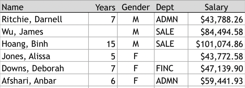
The default row identifiers are the row indices, consecutive integers that number the rows. However, if there is a column of unique identifiers in the data table, that column can be more usefully designated as the row identifiers. The Name column in the d data table analyzed here is not a variable with data values to analyze but rather an ID field that identifies each row with a unique value for that row. To replace the default integer row labels with the values of the column Name, redefine the status of the corresponding column from a variable to a row identifier.
In the language of relational database, a unique row identifier is a primary key. To save changes to the original data frame, explicitly save the manipulation into a variable or object, such as below, where the change to the d data frame is saved back into the d data frame. If the output of any procedure is not assigned to an object, such as a data frame, the output is directed to the console, where you can view the output, but no changes are saved.
R
Use the lessR function Read() to read the data from an Excel file into an R data frame.1 By default, if Read() detects a file type of .xlsx, it reads the data as an Excel file Read() also displays relevant information about the data that is read into the specified data frame. When reading the data, use the parameter row_names to optionally indicate the column to define as row names. Otherwise, the row names are the consecutive integers.
1 To read an Excel file, Read() relies upon the openxlsx package function read.xlsx(). Base R has no function for reading Excel data.
#d = Read('http://lessRstats.com/data/employee.xlsx', row_names=1)
d <- Read('~/Documents/BookNew/data/Employee/employee.xlsx', row_names=1)
[with the read.xlsx() function from Schauberger and Walker's openxlsx package]
>>> Suggestions
Recommended binary format for data files: feather
Create with Write(d, "your_file", format="feather")
To read a csv or Excel file of variable labelsvar_labels=TRUE
Each row of the file: Variable Name, Variable Label
Read into a data frame named l (the letter el)
More details about your data, Enter: details() for d, or details(name)
Data Types
------------------------------------------------------------
character: Non-numeric data values
integer: Numeric data values, integers only
double: Numeric data values with decimal digits
------------------------------------------------------------
Variable Missing Unique
Name Type Values Values Values First and last values
------------------------------------------------------------------------------------------
1 Years integer 36 1 16 7 NA 7 ... 1 2 10
2 Gender character 37 0 2 M M W ... W W M
3 Dept character 36 1 5 ADMN SALE FINC ... MKTG SALE FINC
4 Salary double 37 0 37 53788.26 94494.58 ... 56508.32 57562.36
5 JobSat character 35 2 3 med low high ... high low high
6 Plan integer 37 0 3 1 1 2 ... 2 2 1
7 Pre integer 37 0 27 82 62 90 ... 83 59 80
8 Post integer 37 0 22 92 74 86 ... 90 71 87
------------------------------------------------------------------------------------------Now verify the data that has been read.
dim(d)[1] 37 8head(d) Years Gender Dept Salary JobSat Plan Pre Post
Ritchie, Darnell 7 M ADMN 53788.26 med 1 82 92
Wu, James NA M SALE 94494.58 low 1 62 74
Downs, Deborah 7 W FINC 57139.90 high 2 90 86
Hoang, Binh 15 M SALE 111074.86 low 3 96 97
Jones, Alissa 5 W <NA> 53772.58 <NA> 1 65 62
Afshari, Anbar 6 W ADMN 69441.93 high 2 100 100The blank cell in the Excel worksheet is the number of Years worked for James Wu. R represents missing data with the characters NA for Not Available.
Python
Use the Pandas function read_excel() to read data from an Excel file into a Python data frame. Use the parameter index_col to optionally indicate the column to define as row names. Otherwise, the row names are the consecutive integers. The first column in a Pandas data frame is called Column 0.
#df = pd.read_excel('http://lessRstats.com/data/employee.xlsx', index_col=0)
df = pd.read_excel('~/Documents/BookNew/data/Employee/employee.xlsx',
index_col=0)df.shape(37, 8)df.head() Years Gender Dept Salary JobSat Plan Pre Post
Name
Ritchie, Darnell 7.0 M ADMN 53788.26 med 1 82 92
Wu, James NaN M SALE 94494.58 low 1 62 74
Downs, Deborah 7.0 W FINC 57139.90 high 2 90 86
Hoang, Binh 15.0 M SALE 111074.86 low 3 96 97
Jones, Alissa 5.0 W NaN 53772.58 NaN 1 65 62The blank cell in the Excel worksheet is the number of Years worked for James Wu. Python represents missing data with the characters NaN for Not a Number.
Vectors
When working with data, we often wish to specify a collection of multiple values as a single unit, a variable. The values could be data values or values passed to a function to influence its output, such as a list of various colors for the bars in a bar graph.
The term vector is the standard mathematical term for a single, one-dimensional variable with multiple values. Python, however, eschews that standard term, preferring instead the term list.
To subset, we need to know the position of the elements in the data structure, such as data values, we wish to extract. For a vector, identify the position by its ordinal position in the vector, such as the 7th value.
The concept of an index necessarily applies to any data structure. To subset a vector, specify the desired indices within the square brackets, [ ] immediately after the vector’s name.
The distinction, as always, is that R starts counting from 1 and Python starts from 0.
R
Create
The most general form for specifying an R vector is the c() function for combine. For example, define a vector of the first five integers beginning with 1.
c(1,2,3,4,5)[1] 1 2 3 4 5When a vector is created, its values are usually assigned to a specific variable or parameter. Here, assign the values of the vector to any chosen variable, such as x, as in this example.
x <- c(1,2,3,4,5)
x
[1] 1 2 3 4 5For the particular case of sequential values, two shortcuts are available. One shortcut is the : notation for sequential integers.
1:5[1] 1 2 3 4 5The seq() function defines any regular sequence of values. To use seq(), specify three values: the beginning value, the ending value, and the interval between the values specified with the parameter by.
seq(1, 5, by=1)[1] 1 2 3 4 5We also can have vectors with character values.
G <- c("Man", "Woman", "Other")
G
[1] "Man" "Woman" "Other"One common use of vectors is passing multiple values to the parameters of a function. This example shows a bar chart with customized colors instead of relying upon the default colors. Specify the interior of each of the two bars with a different color by setting the fill parameter to a vector. Specify the exterior of each bar, the border color, with the color parameter, again set to a vector, one color per bar.
As done here, we can enter the vectors into the function call to lessR BarChart() directly or store them as separate variables.
inside <- c("cadetblue", "darkseagreen")
edge <- c("black", "black")
BarChart(Gender, fill=inside, color=edge, data=d, quiet=TRUE)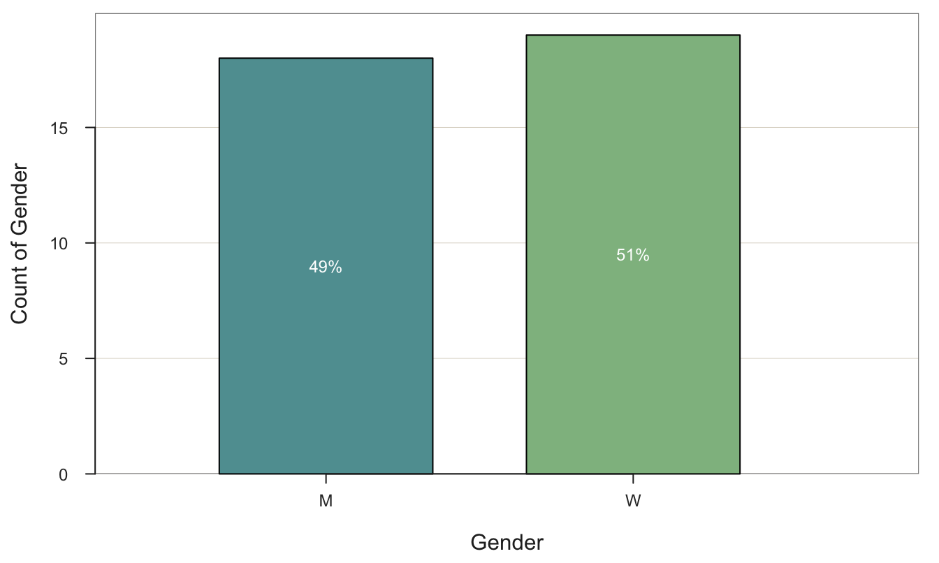
A special operator determines if a value is included in a vector.
An example of an R vector implicitly present in every data analysis is the vector of variable names for a data frame containing the data for analysis. The data frame is a two-dimensional table, but the names of the variables in the data frame, obtained from the Base R names() function, is a vector. In this example, read the data into the data frame named d.
names(d)[1] "Years" "Gender" "Dept" "Salary" "JobSat" "Plan" "Pre" "Post" Here, we see that Salary is a name in the vector of names for the d data frame, but xxx is not.
"Salary" %in% names(d)[1] TRUE"xxx" %in% names(d)[1] FALSESubset
Suppose you wish to change the name of the seventh variable in the Employee data frame. Here, display the name of the seventh variable.
names(d)[7][1] "Pre"Now, change the name of the seventh variable in the names(d) vector from Pre to the more descriptive PreTest.
names(d)[7] <- "PreTest"
names(d)
[1] "Years" "Gender" "Dept" "Salary" "JobSat" "Plan" "PreTest" "Post" Python
Create
A list is a fundamental Python data structure defined as a sequence of multiple items separated by commas. Unlike the R vector, the elements of a list need not be of the same data type. Define a list with the elements enclosed within square brackets, [ ] , here the values are the integers from 1 to 5, inclusive.
[1,2,3,4,5][1, 2, 3, 4, 5]The Python range() function defines a regular sequence of values. To use range(), specify three values: the beginning value, a number past the ending value, and the interval between the values. Here, to specify the numbers from 1 to 5, specify 6 as the ending value. Also, to save memory, unlike the corresponding R function, range() does not produce the values in the sequence all at once but rather one at a time. To illustrate its use, to view the output, we need to specify a loop that generates each value of the sequence, one at a time, and then print the resulting values.
for i in range(1,6,1):
    print(i, end=" ")
1 2 3 4 5 List character string values in quotes when referencing them. Here, assign the list to a variable and display its contents.
G = ["Man", "Woman", "Other"]
G
['Man', 'Woman', 'Other']We can enter the vectors, each as a Python list, into the function call to the seaborn countplot() function directly or store them as separate variables, as done here. The parameter palette specifies the interior color of the bars, and edgecolor specifies the exterior, the edge color.
import seaborn as sns
inside = ["cadetblue", "darkseagreen"]
edge = ["black", "black"]
sns.countplot(data=df, x='Gender', palette=inside, edgecolor=edge)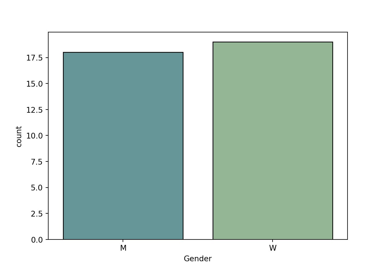
An example of a Python list implicitly present in every data analysis is the vector of variable names for a data frame containing the data for analysis The data frame is a two-dimensional table, but the names of the variables in the data frame, obtained from the Pandas columns method, is just one dimension. In this example, read the data into the data frame named df.
df.columnsIndex(['Years', 'Gender', 'Dept', 'Salary', 'JobSat', 'Plan', 'Pre', 'Post'], dtype='object')Using the in operator, we see that Salary is a name in the vector of names for the d data frame, but xxx is not.
'Salary' in df.columnsTrue'xxx' in df.columnsFalseSubset
df.columns.valuesarray(['Years', 'Gender', 'Dept', 'Salary', 'JobSat', 'Plan', 'Pre',
'Post'], dtype=object)To change the name of the 7th variable, Pre, to PreTest, refer to the 6th index value.
df.columns.values[6] = "PreTest"
df.columns.values
array(['Years', 'Gender', 'Dept', 'Salary', 'JobSat', 'Plan', 'PreTest',
'Post'], dtype=object)Subset a Data Frame
Introduction
Two General Techniques
Subsetting is an essential data preparation process. From a collection of data values, such as a data frame, you may only want to analyze some of them, a subset of the original data. Subset a data frame by rows, by columns, or simultaneously by both. Of course, to perform the subset, the relevant rows and columns of the data frame must first be identified.
There are two basic ways to subset a data frame: Using the Extract procedure or a standard function. Both methods are frequently used, so everyone should be aware of both, even if preferring one method. The Extract procedure is described first.
But before that description, consider a conceptual difference between R and Pandas for creating new data frames from existing data frames.
Deep Copy
When subsetting a data frame or copying the complete data frame, you often want to save the result to a new data frame for further analysis. For example, copy the d data frame to the dNew data frame with the following expression, which works in both R and Python, though in R we usually use <- for the assignment operator.
dNew = dFor such a copy, R actually makes a copy such that there are now two data frames, separate from each other: d and dNew. Pandas, however, does not make a copy from the above expression. A weird Pandas quirk, by default, is that the data values in the new data frame refer to the same memory locations as the original data. The subsetted data in a new data frame remains linked to the original, called a shallow copy, but not a copy at all, just a set of links. If you subsequently modify dNew, the original data frame, the corresponding values in d will also be modified. To keep the copy distinct from the original, the R default, add the copy() function at the end of the subset or copy statement, as in .copy(), creating what pandas calls a deep copy, which is actually just a regular copy.
dNew = d.copy()Unlike R, only with this modified expression do you have a dNew data frame that is its own entity, able to exist independently of the original d data frame. Weird but true. In my opinion, the default should be a deep copy, as with R, and if memory needs to be saved, then add the option for a linked copy. Either change the default or use a different operator than = for both a set of links and an actual copy. Lack of conciseness is never a good outcome when using computers, and this ambiguity is one of the “gotchas” for new Python programmers.
Extract Function
The 2-dimensional data frame has both rows and columns. Accordingly, to identify a subset of a data frame, we need to identify the rows and columns to be included (or excluded) from the data frame. The general form of the Extract subsetting expression for R and Pandas, here shown for the data frame name d:
d[rows, columns]
The rows specifications come before the comma, and the columns specifications come after the comma. For R, the comma must always be present. If no rows or no columns are specified, then all rows or all columns are indicated.
For data frame d, express the rows and columns of the Extract function
d[rows, cols]with either indices or logical expressions.
An example of a set of indices is 1:3, the first three rows using R. An example of a logical expression is Gender=="Man", where the two equal signs indicate to check for equality of existing values. Each method is considered separately below.
Subset by Index
One method to identify a data frame row or column is by its ordinal position within the data frame, its index as previously defined for vectors. Regarding data frames, there is both a row and a column index.
R
Entering the name of an R object, such as the data frame d, implicitly invokes the R print() function, which displays the entire contents of the object at the console. Using the subset notation, selected pieces of the object can be displayed instead. In this example, display the first three rows of data for all the variables.
d[1:3,] Years Gender Dept Salary JobSat Plan Pre Post
Ritchie, Darnell 7 M ADMN 53788.26 med 1 82 92
Wu, James NA M SALE 94494.58 low 1 62 74
Downs, Deborah 7 W FINC 57139.90 high 2 90 86We need to know the column numbers for the specified variables to select variables by column position. Display the column indices with the lessR details_brief() function, abbreviated db(), the same function Read() calls to display information when reading data into a data frame. The variables are numbered from 1 to the last variable. As usual, with lessR, the default data frame is d, otherwise, specify the name of the data frame in the call to db().
db(d)Data Types
------------------------------------------------------------
character: Non-numeric data values
integer: Numeric data values, integers only
double: Numeric data values with decimal digits
------------------------------------------------------------
Variable Missing Unique
Name Type Values Values Values First and last values
------------------------------------------------------------------------------------------
1 Years integer 36 1 16 7 NA 7 ... 1 2 10
2 Gender character 37 0 2 M M W ... W W M
3 Dept character 36 1 5 ADMN SALE FINC ... MKTG SALE FINC
4 Salary double 37 0 37 53788.26 94494.58 ... 56508.32 57562.36
5 JobSat character 35 2 3 med low high ... high low high
6 Plan integer 37 0 3 1 1 2 ... 2 2 1
7 Pre integer 37 0 27 82 62 90 ... 83 59 80
8 Post integer 37 0 22 92 74 86 ... 90 71 87
------------------------------------------------------------------------------------------Column references follow the comma in the Extract expression. Here, display the first two rows of data for the first, second, third, and sixth variables. If all rows are to be retained, enter no information before the comma.
d[1:2, c(1:3, 6)] Years Gender Dept Plan
Ritchie, Darnell 7 M ADMN 1
Wu, James NA M SALE 1Explicitly refer to the column numbers to delete with a - sign. Here, delete the variables Pre and Post, where Pre and Post are in Columns 7 and 8. Show for just the first three rows of data.
d[1:3, -(7:8)] Years Gender Dept Salary JobSat Plan
Ritchie, Darnell 7 M ADMN 53788.26 med 1
Wu, James NA M SALE 94494.58 low 1
Downs, Deborah 7 W FINC 57139.90 high 2Python
Unfortunately, in my opinion, unlike the way we usually count, Python, and so Pandas, is zero-indexed, which means that it begins counting at 0 instead of 1. Yes, Python labels the second row of data as Row 1. And the first row is Row 0. Using Python, all you can do is get used to it, #1 is really #2.
Related to this zero-indexing property, Python subsets exclusive of the ending index. When specifying a range of indices, such as from 0 to 2 in this example, you need to specify one additional integer beyond the numbers that are read. Again, get used to it with Python, which works hard to avoid just simple numbering from 1 to whatever, such as with R. If you want to specify the first three rows of data — 0, 1, and 2 — specify rows from 0 to 3.
The Pandas world presents two ways to subset a data frame by rows, with and without the iloc method, for integer location. You will encounter both methods in reading other people’s code. For reference, here is a subset of the first three rows without the method.
df[0:3] Years Gender Dept Salary JobSat Plan Pre Post
Name
Ritchie, Darnell 7.0 M ADMN 53788.26 med 1 82 92
Wu, James NaN M SALE 94494.58 low 1 62 74
Downs, Deborah 7.0 W FINC 57139.90 high 2 90 86However, if subsetting by rows and columns, then iloc must be invoked, but can be used just for rows as well, as shown here. If only subsetting rows, then the comma from which the columns would be specified is not needed.
df.iloc[0:3] Years Gender Dept Salary JobSat Plan Pre Post
Name
Ritchie, Darnell 7.0 M ADMN 53788.26 med 1 82 92
Wu, James NaN M SALE 94494.58 low 1 62 74
Downs, Deborah 7.0 W FINC 57139.90 high 2 90 86Next, subset by rows and by columns. To specify a range of columns that is not contiguous, enter the multiple index numbers as a list. A list is also defined by [ ], so these brackets are arranged one set nested in the other. Here, display the first two rows of data for the first, second, third, and sixth variables.
df.iloc[0:2, [0,1,2, 5]] Years Gender Dept Plan
Name
Ritchie, Darnell 7.0 M ADMN 1
Wu, James NaN M SALE 1Columns (or rows) can also be deleted by using the drop() function. The axis=1 refers to columns and is needed even though the reference is already set to columns.
df2 = df.drop(df.columns[[6,7]], axis=1)
df2.iloc[0:3, :]
Years Gender Dept Salary JobSat Plan
Name
Ritchie, Darnell 7.0 M ADMN 53788.26 med 1
Wu, James NaN M SALE 94494.58 low 1
Downs, Deborah 7.0 W FINC 57139.90 high 2Subset by Criteria
Retrieve just those rows of data that match a logical condition. Here, identify all rows of data for employees with a Salary of more than $100,000 per year. The first example only displays the result. The second example creates a new data frame with the result and then displays the subset data frame.
R
Rows
For example, consider d$Gender and d$Salary when subsetting the d data frame by Gender and Salary. Here, subset only men with salaries above $100,000, retaining all the variables. That is, extract only those rows where the variable Gender is equal to “M” and the variable Salary is greater than $100,000.
d[d$Salary > 100000, ] Years Gender Dept Salary JobSat Plan Pre Post
Hoang, Binh 15 M SALE 111074.9 low 3 96 97
Correll, Trevon 21 M SALE 134419.2 low 1 97 94
James, Leslie 18 W ADMN 122563.4 low 3 70 70
Capelle, Adam 24 M ADMN 108138.4 med 2 83 81Applied to the Base R Extract function, the lessR function .() simplifies the expression by eliminating the need to pre-pend the data frame name and a $ to each variable name in the specified logical expression to select rows. This pre-pending should not be necessary because the system already knows the relevant data frame, which is d in this example.
d[.(Salary > 100000), ] Years Gender Dept Salary JobSat Plan Pre Post
Hoang, Binh 15 M SALE 111074.9 low 3 96 97
Correll, Trevon 21 M SALE 134419.2 low 1 97 94
James, Leslie 18 W ADMN 122563.4 low 3 70 70
Capelle, Adam 24 M ADMN 108138.4 med 2 83 81Here, query all men in Finance. The ampersand, &, indicates “and”. Because the entire expression is enclosed in single quotes, ' , enclose character constants within the string with double quotes, ".
d[.(Dept == "FINC" & Gender == "M"), ] Years Gender Dept Salary JobSat Plan Pre Post
Sheppard, Cory 14 M FINC 95027.55 low 3 66 73
Link, Thomas 10 M FINC 66312.89 low 1 83 83
Cassinelli, Anastis 10 M FINC 57562.36 high 1 80 87To select rows by row names if they exist beyond the consecutive integers, invoke the Base R function rownames(), referencing the data frame, here d. If selecting more than a single row, express the row names as a vector and use %in% in place of double equals, ==. Again, no variables are specified after the comma, so all variables are retained in the subset.
d[rownames(d) %in% c("Hoang, Binh", "Downs, Deborah"), ] Years Gender Dept Salary JobSat Plan Pre Post
Downs, Deborah 7 W FINC 57139.9 high 2 90 86
Hoang, Binh 15 M SALE 111074.9 low 3 96 97Columns
The Base R Extract function presents two annoying features for variable selection. First, to select specific variables, all variable names must be between quotes. Second, only individual variables can be specified, more than one variable as a vector with the c() function. Specify variable ranges of contiguous variables by a colon, :, are not permitted. The lessR function .() addresses these deficiencies. No quotes are required around the variable names, and as many variable ranges and single variables as desired may be specified in a single function call.
Here, specify all variables in the d data frame of the Employee data starting with Years through Salary, and also add the variable Post to the specification.
d[1:3, .(Years:Salary, Post)] Years Gender Dept Salary Post
Ritchie, Darnell 7 M ADMN 53788.26 92
Wu, James NA M SALE 94494.58 74
Downs, Deborah 7 W FINC 57139.90 86To indicate that the specified variables should be excluded instead of included, add a minus sign, -, preceding the .() function call.
d[1:3, -.(Years:Salary, Post)] JobSat Plan Pre
Ritchie, Darnell med 1 82
Wu, James low 1 62
Downs, Deborah high 2 90The R Extract function has the annoying characteristic of returning a vector instead of a data frame if only one variable is retained.
d[1:3, .(Salary)][1] 53788.26 94494.58 57139.90To retain the status of a data frame when only a single variable remains after the subset, set the drop parameter to FALSE.
d[1:3, .(Salary), drop=FALSE] Salary
Ritchie, Darnell 53788.26
Wu, James 94494.58
Downs, Deborah 57139.90Python
Rows
To specify a logical criterion by which to select rows using extract, identify the variable as existing within a data frame. Instead of .iloc, use the .loc method for specifying a logical criterion.
df.loc[df['Salary'] > 100000, :] Years Gender Dept Salary JobSat Plan Pre Post
Name
Hoang, Binh 15.0 M SALE 111074.86 low 3 96 97
Correll, Trevon 21.0 M SALE 134419.23 low 1 97 94
James, Leslie 18.0 W ADMN 122563.38 low 3 70 70
Capelle, Adam 24.0 M ADMN 108138.43 med 2 83 81Here, query all Men in Finance. The ampersand, &, indicates “and”. When specifying multiple criteria, enclose each criterion within parentheses.
df.loc[(df['Dept'] == 'FINC') & (df['Gender'] == 'M'), :] Years Gender Dept Salary JobSat Plan Pre Post
Name
Sheppard, Cory 14.0 M FINC 95027.55 low 3 66 73
Link, Thomas 10.0 M FINC 66312.89 low 1 83 83
Cassinelli, Anastis 10.0 M FINC 57562.36 high 1 80 87To select rows by row names if they exist beyond the consecutive integers, invoke the loc method. If selecting more than a single row, express the row names as a list, defined by the row names enclosed within [ ].
df.loc[['Hoang, Binh', 'Downs, Deborah'], :] Years Gender Dept Salary JobSat Plan Pre Post
Name
Hoang, Binh 15.0 M SALE 111074.86 low 3 96 97
Downs, Deborah 7.0 W FINC 57139.90 high 2 90 86Columns
Here, specify all variables in the df data frame of the Employee data starting with Years through Salary, and also add the variable Post to the specification. This expression is more complicated than the corresponding R, and especially lessR. Also, unlike R, we cannot mix row indices and variable names, so we separate to display only the first three rows of subsetted data.
The easiest in Pandas to specify columns is to list each variable name separately.
d2 = df.loc[:, ['Years', 'Gender', 'Dept', 'Salary', 'Post']]
d2.iloc[0:3, :]
Years Gender Dept Salary Post
Name
Ritchie, Darnell 7.0 M ADMN 53788.26 92
Wu, James NaN M SALE 94494.58 74
Downs, Deborah 7.0 W FINC 57139.90 86Of course, listing each name separately can be tedious. Following is an example of using a cell range, which is straightforward enough, but becomes more complicated when variables outside of that cell range are variables to also be included in the subset. Here, use the join() function, which adds more variables to the data frame defined by the initially specified range of variables.
d2 = df.loc[:, 'Years':'Salary'].join(df['Post'])
d2.iloc[0:3, :]
Years Gender Dept Salary Post
Name
Ritchie, Darnell 7.0 M ADMN 53788.26 92
Wu, James NaN M SALE 94494.58 74
Downs, Deborah 7.0 W FINC 57139.90 86This expression to delete a range of variables and a variable outside of that range is way more complicated than the corresponding R, and especially lessR, expressions. The list() function is direct from the core Python. The function creates a list (vector) without the square brackets [ ].
df2 = df.drop(columns=
      list(df.loc[:, 'Years':'Salary'].columns) + ['Post'])
df2.iloc[0:3, :]
JobSat Plan Pre
Name
Ritchie, Darnell med 1 82
Wu, James low 1 62
Downs, Deborah high 2 90General Functions
The two general methods for subsetting data are the Extract method previously described and specific functions of the usual form written to accomplish specific types of subsetting. General subsetting functions are presented in this section, which generally work by specifying logical conditions for selecting rows and columns of a data frame.
R
Rows of data from the data table can be selected according to logical criteria. The retained rows of data are those that fulfill the criteria. Use ! for not. To relate two different criteria, use & for and | for or. For exclusive pairing, one of two criteria is true but not both, invoke the xor function, as in xor(x, y).
Base R provides the subset() function. The first parameter value specifies the logical criteria for the rows and is weirdly named with the same name of the function, subset. However, because it is listed first in the function definition, it is unnecessary to include the parameter name in the function call. The second parameter is select, which specifies logical criteria for selecting columns.
Rows
Following the previous example, select all Men who work in Finance.
subset(d, Dept == "FINC" & Gender == "M") Years Gender Dept Salary JobSat Plan Pre Post
Sheppard, Cory 14 M FINC 95027.55 low 3 66 73
Link, Thomas 10 M FINC 66312.89 low 1 83 83
Cassinelli, Anastis 10 M FINC 57562.36 high 1 80 87Columns
This example uses the Base R subset() function with the select parameter, selecting two variables from the data frame. To minimize the display, save the result into another data frame and then only show the first three rows.
d2 <- subset(d, select=c(Pre, Post))
d2[1:3, ]
Pre Post
Ritchie, Darnell 82 92
Wu, James 62 74
Downs, Deborah 90 86Or, delete the two variables from the data frame with a - sign before of the vector of variable names.
d2 <- subset(d, select=-c(Pre, Post))
d2[1:3, ]
Years Gender Dept Salary JobSat Plan
Ritchie, Darnell 7 M ADMN 53788.26 med 1
Wu, James NA M SALE 94494.58 low 1
Downs, Deborah 7 W FINC 57139.90 high 2Defining an R vector of names is straightforward, even with a range of variable names and a variable outside of that range.
d2 <- subset(d, select=c(Gender:Salary, Pre))
d2[1:3, ]
Gender Dept Salary Pre
Ritchie, Darnell M ADMN 53788.26 82
Wu, James M SALE 94494.58 62
Downs, Deborah W FINC 57139.90 90Python
Rows
This first example invokes the most straightforward method of selecting rows satisfying a logical condition: The query() function. Enclose the logical condition in quotes.
df.query('Salary > 100000') Years Gender Dept Salary JobSat Plan Pre Post
Name
Hoang, Binh 15.0 M SALE 111074.86 low 3 96 97
Correll, Trevon 21.0 M SALE 134419.23 low 1 97 94
James, Leslie 18.0 W ADMN 122563.38 low 3 70 70
Capelle, Adam 24.0 M ADMN 108138.43 med 2 83 81Here, query all Men in Finance. The ampersand, &, indicates “and”. Because the entire expression is enclosed in single quotes, ' , enclose character constants within the string with double quotes, ".
df.query('Dept == "FINC" & Gender == "M"') Years Gender Dept Salary JobSat Plan Pre Post
Name
Sheppard, Cory 14.0 M FINC 95027.55 low 3 66 73
Link, Thomas 10.0 M FINC 66312.89 low 1 83 83
Cassinelli, Anastis 10.0 M FINC 57562.36 high 1 80 87Columns
Use the filter() function to select columns. To minimize the display, save the result into another data frame and then only show the first three rows.
d2 = df.filter(['Pre', 'Post'])
d2[0:3]
Pre Post
Name
Ritchie, Darnell 82 92
Wu, James 62 74
Downs, Deborah 90 86Drop variables, columns in the data frame, with the drop() function.
d2 = df.drop(['Pre', 'Post'], axis="columns")
d2[0:3]
Years Gender Dept Salary JobSat Plan
Name
Ritchie, Darnell 7.0 M ADMN 53788.26 med 1
Wu, James NaN M SALE 94494.58 low 1
Downs, Deborah 7.0 W FINC 57139.90 high 2Compare the complexity with Pandas of dropping of variables in a range plus a variable outside of that range with the simplicity of creating an R vector that defines those variables.
d2 = df.drop(
  columns=list(df.loc[:, 'Years':'Salary'].columns) + ['Post'])
d2[0:3]
JobSat Plan Pre
Name
Ritchie, Darnell med 1 82
Wu, James low 1 62
Downs, Deborah high 2 90Chained Functions
When multiple operations need to be performed on a data frame, the elegant solution is to combine all the operations into a single, unified statement. Both R and Python provide for this unification.
R
The Pipe Operator
Stefan Milton’s magrittr 2014 package of the same name introduced the forward pipe (or chain) operator, %>%, pronounced then. The operator transformed how many people code their data transformations by organizing them as a flow from start to end.
Milton’s creation of the pipe operator was sufficiently profound that the Tidyverse R people adopted it into their system. They did so quickly after its appearance to the extent that I think many people today falsely attribute its invention to the Tidyverse people. Moreover, the popularity of the operator eventually incentivized the R people to adopt their own version of the operator into Base R since R 4.1.0. The Base R pipe operator is |>. I use the Base R version because I usually do not have the Tidyverse packages or the magrittr package attached to my R analysis and |> is automatically available. Although with more advanced uses %>% and |> have some distinctions, at their basic use the operators are interchangeable.
By default, the forward pipe operator takes the output from the preceding function in the chain and inputs that previous output into the first parameter of the subsequent function.
When a data frame is passed from the function on the left of the operator to the function on the right, if the data frame is the first parameter in the function definition, it is not specified in the function call.
A simple example for illustration purposes only is the head() function, which has the input data frame as its first parameter, normally written as head(d) for the d data frame. Here, the data frame d is piped into the first parameter value of the head() function, the data structure.
d |> head() Years Gender Dept Salary JobSat Plan Pre Post
Ritchie, Darnell 7 M ADMN 53788.26 med 1 82 92
Wu, James NA M SALE 94494.58 low 1 62 74
Downs, Deborah 7 W FINC 57139.90 high 2 90 86
Hoang, Binh 15 M SALE 111074.86 low 3 96 97
Jones, Alissa 5 W <NA> 53772.58 <NA> 1 65 62
Afshari, Anbar 6 W ADMN 69441.93 high 2 100 100Use a placeholder to pipe the data into another parameter other than the function’s first parameter. For the Base R pipe, the _ serves as a placeholder for the piped-in incoming information and must be accompanied by the parameter name. For the magrittr pipe operator, %>%, the placeholder is a period, ..
The following example is a bit more convoluted than the traditional function call but illustrates that the _ can be the receiver of information passed to any parameter. Forward the constant 2 into the head() function as the value of n, the number of lines to display for the input data frame.
2 |> head(d, n=_) Years Gender Dept Salary JobSat Plan Pre Post
Ritchie, Darnell 7 M ADMN 53788.26 med 1 82 92
Wu, James NA M SALE 94494.58 low 1 62 74Because the Base R operator is part of R, no external packages need be referenced for its pipe operator. That said, the magrittr pipe operator was first, so its use is quite common by R users. For basic operations, such as shown here, either version of the pipe works equally well. With Version 4 of R, the R people followed Milton’s lead and introduced the Base R pipe operator, |>, used in the following example.
Obtain the pipe operator directly from the keyboard within RStudio as CNTRL/CMD-SHIFT-M. The default pipe operator is %>%. However, this default can be changed with a trip to:
- RStudio’s Tools –> Global Options…
- Select Code followed by the Editing tab, then the relevant check box
Checking the relevant check box changes the default pipe operator to the Base R |>.
Realistic Examples
This example subsets rows and then columns and then sorts the resulting subsetted data frame in descending order of Salary with the lessR function sort_by.
d |>
  subset(Salary > 100000) |>
  subset(select=c(Gender, Salary)) |>
  sort_by(Salary, direction="-")
Sort Specification
  Salary -->  descending
Gender Salary
Correll, Trevon M 134419.2
James, Leslie W 122563.4
Hoang, Binh M 111074.9
Capelle, Adam M 108138.4Or, use the Extract function to subset, combining the row and column selection into a single statement plus the convenience of the lessR function .(). Go one step further and save the sorted, subsetted data frame into the created data frame a. Do so by adding the following assignment statement to the end of the chained function calls: -> a. In this case, the object on the right is assigned the contents of the object on the left of the operator in the reverse order in which the assignment operator is usually written.
d[.(Salary > 100000), .(Gender, Salary)] |>
  sort_by(Salary, direction="-") ->
a
Sort Specification
Salary --> descending head(a) Gender Salary
Correll, Trevon M 134419.2
James, Leslie W 122563.4
Hoang, Binh M 111074.9
Capelle, Adam M 108138.4Using the assignment operator in that direction maintains the flow of information in the piped function calls from left to right, top to bottom.
Python
When doing multiple function calls, one after the other, you can chain query() and filter() functions and other functions into a single statement. Chaining results in a multi-step data manipulation process with highly readable, structured code. Specify a set of chained functions, each on their own line to enhance readability. Include the entire expression within parentheses ( ).
In this example, subset by rows with query(), then by columns with filter(), then sort on the Salary column with the Pandas function sort_values()`.
(df
  .query('Salary > 100000')
  .filter(['Gender', 'Salary'])
  .sort_values(['Salary'], ascending=False)
)
Gender Salary
Name
Correll, Trevon M 134419.23
James, Leslie W 122563.38
Hoang, Binh M 111074.86
Capelle, Adam M 108138.43This example subsets rows, then columns. After subsetting, sort the resulting data frame in descending order of Salary with the Pandas function sort_values().
Variable Transformation
Variables are continuous or categorical. Continuous variables are numerical. Categorical variables are usually stored digitally as either integers or character strings, and then converted to a variable of type factor for R and type category for Pandas. As with most analyses, the procedure of variable transformation differs for continuous and categorical variables.
Continuous Variables
To transform the values of a continuous variable is straightforward: Enter and process the corresponding equation that defines the transformation. The Excel analogy to create a transformed variable is to enter the equation in the top cell of the column of data values and then: Fill --> Down.When entering this equation in R or Python, remember when referring to a variable contained within a date frame to include the data frame along with the variable name. This reference is done differently in R and Python as illustrated below.
R
Refer to a variable within a data frame with the data frame name, such as d, and then a $ followed by the variable name. For example, refer to the Salary variable in the d data frame as d$Salary.
Here, create a new variable, Salary000, defined as the original Salary variable with values divided by 1000, rounded to two decimal digits with the Base R round() function. The new variable is added to the existing variables in the d data frame. Processing the equation creates the values of the new variable for all rows of data in the data frame.
d$Salary000 <- round(d$Salary / 1000, 2)
head(d)
Years Gender Dept Salary JobSat Plan Pre Post Salary000
Ritchie, Darnell 7 M ADMN 53788.26 med 1 82 92 53.79
Wu, James NA M SALE 94494.58 low 1 62 74 94.49
Downs, Deborah 7 W FINC 57139.90 high 2 90 86 57.14
Hoang, Binh 15 M SALE 111074.86 low 3 96 97 111.07
Jones, Alissa 5 W <NA> 53772.58 <NA> 1 65 62 53.77
Afshari, Anbar 6 W ADMN 69441.93 high 2 100 100 69.44Using the same variable name on both sides of the equation replaces the original with the transformed version.
Python
Refer to a variable within a data frame with the data frame name, such as df, and then the variable name within quotes and square brackets. For example, refer to the Salary variable in the df data frame: df[‘Salary’].
Here, create a new variable, Salary000, defined as the original Salary variable with values divided by 1000, rounded to two decimal digits. The new variable is added to the existing variables in the d data frame. Running the equation creates the values of the new variable for all rows of data in the data frame. Using the same variable name on both sides of the equation replaces the original with the transformed version.
df['Salary000'] = round(df['Salary'] / 1000, 2)
df.head()
Years Gender Dept Salary ... Plan Pre Post Salary000
Name ...
Ritchie, Darnell 7.0 M ADMN 53788.26 ... 1 82 92 53.79
Wu, James NaN M SALE 94494.58 ... 1 62 74 94.49
Downs, Deborah 7.0 W FINC 57139.90 ... 2 90 86 57.14
Hoang, Binh 15.0 M SALE 111074.86 ... 3 96 97 111.07
Jones, Alissa 5.0 W NaN 53772.58 ... 1 65 62 53.77
[5 rows x 9 columns]Categorical Variables
Unlike a continuous variable, to transform the values of categorical variables without a general equation is to specify how each level or category should be transformed. For the Employee data set, the categorical variables are the integer coded Plan and the character string variables Gender, Dept, and JobSat.
R
As previously described, convert categorical variables to R factors. For a character string variable this conversion can be used to relabel the levels of the variable, its data values. Here, replace any M or W for the variable Gender with Man and Woman as displayed in the output, both text and data visualizations. The values stored in the factor variable are just the integers 1 and 2 in this example with two levels. After the conversion, show just the first six rows of the data frame and the values for the character string variable Gender and the factor G.
d$G <- factor(d$Gender, levels=c("M", "W"),
                        labels=c("Man", "Woman"))
d[1:6, .(Gender, G)]
Gender G
Ritchie, Darnell M Man
Wu, James M Man
Downs, Deborah W Woman
Hoang, Binh M Man
Jones, Alissa W Woman
Afshari, Anbar W WomanHowever, the actual data values, the levels, can be changed in the data frame with the lessR function recode(), which recodes individual values of a categorical variable. Parameter old indicates the values to be replaced, and parameter new indicates the replacement value.
After the transformation, show the first six rows of data and all variables from Years to Salary in the data frame. The output of recode() is to a data frame. In this example, create a new data frame, d2, leaving the original version, d, unmodified.
d2 <- recode(Gender, old=c("M", "W"),
                     new=c("Man", "Woman"), data=d)
--------------------------------------------------------
First four rows of data to recode for data frame: d
--------------------------------------------------------
                 Gender
Ritchie, Darnell      M
Wu, James             M
Downs, Deborah        W
Hoang, Binh           M


Recoding Specification
----------------------
   M --> Man
   W --> Woman

Number of cases (rows) to recode: 37

Replace existing values of each specified variable, no value for option: new.var

---  Recode: Gender ---------------------------------
Number of unique values of Gender in the data: 2
Number of values of Gender to recode: 2


------------------------------------------------
First four rows of recoded data
------------------------------------------------
                 Gender
Ritchie, Darnell    Man
Wu, James           Man
Downs, Deborah    Woman
Hoang, Binh Mand2[1:6, .(Years:Salary)] Years Gender Dept Salary
Ritchie, Darnell 7 Man ADMN 53788.26
Wu, James NA Man SALE 94494.58
Downs, Deborah 7 Woman FINC 57139.90
Hoang, Binh 15 Man SALE 111074.86
Jones, Alissa 5 Woman <NA> 53772.58
Afshari, Anbar 6 Woman ADMN 69441.93The data parameter is not needed in the previous function call to recode() because the corresponding data frame is d, which is the default data frame name for lessR functions. However, the parameter can still be specified to explicitly show the data frame that is being accessed for this function call.
Now that the data values in the data frame for Gender are replaced with their new values, still consider converting Gender to a factor variable. For example, the value of Other may not have occurred in such a small data sample of 37 employees, but to include Other in the results, such as a bar chart, that level would be declared when converting to a variable of type factor.
Python
The Pandas function replace() recodes individual values of a categorical variable. Parameter to_replace indicates the values to be replaced, and parameter value indicates the replacement value. Here, recode with replace() replaces any ‘M’ and ‘W’ in the entire data table, which turns out to be just for the values of Gender.
d_obj = df.replace(to_replace=['W', 'M'],
                        value=['Woman', 'Man'])
d_obj.head()
Years Gender Dept Salary ... Plan Pre Post Salary000
Name ...
Ritchie, Darnell 7.0 Man ADMN 53788.26 ... 1 82 92 53.79
Wu, James NaN Man SALE 94494.58 ... 1 62 74 94.49
Downs, Deborah 7.0 Woman FINC 57139.90 ... 2 90 86 57.14
Hoang, Binh 15.0 Man SALE 111074.86 ... 3 96 97 111.07
Jones, Alissa 5.0 Woman NaN 53772.58 ... 1 65 62 53.77
[5 rows x 9 columns]This following use of replace() targets only values of the variable Gender. The curly brackets { and } indicate a specific Python data type called a dictionary. As with any dictionary, there is a keyword followed by the meaning. For example, the keyword ‘F’ has the meaning ‘Woman’. The advantage of replacing categorical values with a dictionary is that each replacement is explicitly paired with the original value. The variable Gender has values ‘F’ and ‘M’, here replaced with ‘Woman’ and ‘Man’, respectively.
dd = df.replace({'Gender': {'W': 'Woman', 'M': 'Man'}}).copy()
dd.head()
Years Gender Dept Salary ... Plan Pre Post Salary000
Name ...
Ritchie, Darnell 7.0 Man ADMN 53788.26 ... 1 82 92 53.79
Wu, James NaN Man SALE 94494.58 ... 1 62 74 94.49
Downs, Deborah 7.0 Woman FINC 57139.90 ... 2 90 86 57.14
Hoang, Binh 15.0 Man SALE 111074.86 ... 3 96 97 111.07
Jones, Alissa 5.0 Woman NaN 53772.58 ... 1 65 62 53.77
[5 rows x 9 columns]For comparison, here is the original, unmodified data frame df.
df.head() Years Gender Dept Salary ... Plan Pre Post Salary000
Name ...
Ritchie, Darnell 7.0 M ADMN 53788.26 ... 1 82 92 53.79
Wu, James NaN M SALE 94494.58 ... 1 62 74 94.49
Downs, Deborah 7.0 W FINC 57139.90 ... 2 90 86 57.14
Hoang, Binh 15.0 M SALE 111074.86 ... 3 96 97 111.07
Jones, Alissa 5.0 W NaN 53772.58 ... 1 65 62 53.77
[5 rows x 9 columns]As with the R example, this conversion is to the data values in the designated data frame. Regardless, converting the variable to a variable of type category, a formal Pandas categorical variable, provides additional advantages.
Binning
The operation of binning transforms a continuous variable into a categorical variable.
Converting a continuous variable to bins discards information but sometimes the simplification of the data allows for a more understandable presentation, with only a relatively small number of values for the newly defined categorical variable.
One useful set of cut points for defining bins are quantiles of the distribution.
To calculate the quantiles is always in the context of how many equal groups. For example, the median splits a distribution into two groups. Here, we focus on four groups, defined by the 1st, 2nd, and 3rd quartiles.
R
The Base R quantile() function calculates the quantiles of a variable for specified proportions of the distribution. If the distribution is divided into four equal groups, then the distribution’s quartiles are obtained. The data are automatically sorted before the cut points are computed. The values of 0 and 1 in the call to quantile() provide the minimum and maximum Salaries.
cut_points <- quantile(d$Salary, c(0,.25,.50,.75,1))
cut_points
0% 25% 50% 75% 100%
46124.97 56772.95 69547.60 87785.51 134419.23 The quartiles are defined by the three points: $56,772.95, $69,547.6, and $87,785.51. Regarding the lower quartile, 25% of all salaries are lower than $56,772.95, between $46,124.97 and $56,772.95.
The R function cut() bins the specified continuous variable into discrete categories. This example bins according to the quartiles. Specify the cut points with the parameter breaks. The optional labels parameter provides names for the bins. Otherwise, each bin is labeled with its lowest and highest cut point.
The following example creates four bins for the continuous variable Salary, named Low, Med, High, and Top. For example, for the first row of data, Darnell Ritchie has a Salary of $53 USD, which places his value of Salary in the lowest quartile of salaries. His value of Salary_qrt is 1st.
d$Salary_qrt <- cut(d$Salary, breaks=cut_points,
                    labels=c("1st", "2nd", "3rd", "4th"))
head(d)
Years Gender Dept Salary JobSat Plan Pre Post Salary000 G
Ritchie, Darnell 7 M ADMN 53788.26 med 1 82 92 53.79 Man
Wu, James NA M SALE 94494.58 low 1 62 74 94.49 Man
Downs, Deborah 7 W FINC 57139.90 high 2 90 86 57.14 Woman
Hoang, Binh 15 M SALE 111074.86 low 3 96 97 111.07 Man
Jones, Alissa 5 W <NA> 53772.58 <NA> 1 65 62 53.77 Woman
Afshari, Anbar 6 W ADMN 69441.93 high 2 100 100 69.44 Woman
Salary_qrt
Ritchie, Darnell 1st
Wu, James 4th
Downs, Deborah 2nd
Hoang, Binh 4th
Jones, Alissa 1st
Afshari, Anbar 2ndPython
Pandas function qcut(), for quantile cut, bins a continuous variable into discrete categories according to the specified quantiles, the specified cut points at each specified percentage of the distribution. The optional labels parameter provides names for the bins, otherwise the bins are the integers numbered from 0.
The following example creates four bins, the quartiles, for the continuous variable Salary, named Low, Med, High, and Top. For example, for the first row of data, Darnell Ritchie has a Salary of $53 USD, which places his value of Salary in the lowest quartile of salaries. His value of Salary_qrt is 1st.
df['Salary_qrt'] = pd.qcut(df['Salary'], q=[0,.25,.50,.75,1],
                      labels=['1st', '2nd', '3rd', '4th'])
df.head(6)
Years Gender Dept ... Post Salary000 Salary_qrt
Name ...
Ritchie, Darnell 7.0 M ADMN ... 92 53.79 1st
Wu, James NaN M SALE ... 74 94.49 4th
Downs, Deborah 7.0 W FINC ... 86 57.14 2nd
Hoang, Binh 15.0 M SALE ... 97 111.07 4th
Jones, Alissa 5.0 W NaN ... 62 53.77 1st
Afshari, Anbar 6.0 W ADMN ... 100 69.44 2nd
[6 rows x 10 columns]