suppressMessages(library(lessR))
style(suggest=FALSE)The following material is based on the content presented in my book on Pages 22-24 and 43-46:
R Data Analysis without Programming: Explanation and Interpretation, 2nd edition, Routledge, January, 2023.
Introduction
We begin with the fundamental concept, the analysis of data.
All data analysis computations are done today using the computer, yet people analyzed data well before computers were invented. The conceptual meaning of a variable and its data values exists apart from the computer. When stored on the computer, the data values for our variables are represented digitally in computer storage, the data storage type. This distinction applies to all data analysis software.
Whether using R, Python, Excel, or any other system, we need to understand how our data values are digitally stored and how that representation matches our conceptual definitions.
At the most general conceptual level, we have two types of variables. When analyzing data, always distinguish between continuous and categorical variables. At its most general expression, continuous variables are numerical and categorical variables are non-numerical but the more complete expression of this distinction is discussed next.
Two Classes of Variables
Variables are analyzed differently depending on if they are continuous or categorical, so it is essential to know which variables are continuous and which are categorical before beginning any analysis. To complicate the issue more, numbers can represent both types of variables. Moreover, even for continuous variables, the numeric data values can represent different levels of quality, permitting different levels of numerical operations.
Before analysis begins, after reading data into the analysis system, distinguish between the continuous and categorical variables in the data frame and the level of quality of numeric data values.
All of these issues should be understood before analyzing the variables.
Continuous Variables
The values for a continuous variable, sometimes called a quantitative variable, are ordered along a quantitative continuum, the abstraction of the infinitely dense real number line.
Choose any two values and find an unlimited number of numeric values between them. Examples of continuous variables for a person are Age, Salary, and extent of Agreement with an opinion about some political issue; for a car, MPG and Weight; and for a light bulb, Mean Number of Hours until Failure and Electrical Consumption per Hour (kilowatt hours). A continuous variable is sometimes called a quantitative variable.
Distinguish between a continuous variable’s actual values and the data values that emerge from measuring those values.
Measurement categorizes data values into specific groups. The value of the variable as it exists always differs from the value of its measurement, the data value. Nothing, for example, weighs exactly 2 pounds, 2.01 pounds, or even 2.0000000001 pounds. The actual weight may theoretically be stated as an indefinitely large number of decimal digits. In contrast, indicate a measurement to a specific level of precision, such as, for weight, to the nearest pound, ounce, or gram. Measurement groups all similar weights together, approximating the true weight to the nearest pound or whatever.
Interpret the data values measured on a numeric scale for a continuous variable according to one of two types: Ratio data and interval data. Ratio data follow a numeric scale with the usual properties assigned to numbers.
Two different ratio data values can be compared by their ratios: 20 is twice as much as 10. Equal intervals of measurement separate values that are equal distance from each other. For example, the distance between 21 and 22 represents the same underlying difference for 22 and 23.
Just because you have numerical data for a variable does not imply that the data values exhibit the standard properties of numbers on a number line, that is, ratio data. A weaker numerical scale applies to interval data.
Interval data maintains the equal interval property of ratio data but does not have a fixed, natural zero point. The classic example of two alternative interval scales compares Fahrenheit and Celsius temperatures. As an example, compare Fahrenheit and Celsius temperatures. Each temperature scale, for example, has a different value of zero regarding the magnitude of the temperature. 0\(^{\circ}\)F is not the same temperature as 0\(^{\circ}\)C. Ratio comparisons for interval data are not valid; 20\(^{\circ}\)F is not twice as warm as 10\(^{\circ}\)F.
Working with data is, of course, distinct from a mathematician working with theoretical numbers. Working with data reveals four different representations of the values of continuous variables. We store the data on a computer system as a data file and then read the data into an analysis system, such as R or Python. As data analysts, we must ensure that the correct data type in our analysis corresponds to the correct conceptual definition of the variable.
Distinguish between four distinct representations of the values of a variable:
- actual values as they exist apart from their measurement
- data values as recorded measurements of the actual values
- data values stored within a computer file in terms of bits, binary integers
- data values as represented within the analysis system
Categorical Variables
The primary type of variable other than continuous variables is the categorical variable.
Examine the number of unique data values for each variable in the data frame. The values of a categorical variable form a relatively small number of categories called levels. Each level represents a distinct group. For example, the values of the categorical variable Gender define groups of Men, Women, and Other. Other categorical variables are Cola Preference, State of Residence, or Football Jersey Number. Yes, the number on the jersey consists of numeric digits, but those digits are labels, not subject to arithmetic operations such as computing an average. A categorical variable may also be called a qualitative variable or a grouping variable.
The values of categorical variables are labeled rather than measured. We do not measure the state of the USA in which a person resides but instead assign a person to that state based on self-report or an examination of public records. The classification into a group assigns a label, such as Oregon or Texas.
One categorical data type is a set of rankings, called ordinal data, which is data values that are ordered categories.
Suppose the top three sprinters are ranked in order of finish in the 100-meter dash: 1st, 2nd, and 3rd. The finish times represent a continuous variable, but simply ranking contestants by order of their finish does not convey if the race was extremely close or if the winner finished well ahead of their nearest competitor.
Another instance of ordinal data is when the measured value of a continuous variable is so imprecise that, instead of a numerical scale, only a few categories exist in which the measured values can be placed. Suppose that persons admitted to the emergency room are swiftly placed into one of only three severity categories: mild, moderate, or severe. This simple rating scale recognizes that some injuries are more severe than others, but the severity is classified into one of only three categories. The underlying variable for Injury Severity is continuous. This underlying progression of severity is assumed, but not equal intervals of severity that separate the levels. The rater’s interpretation of Moderate Severity of Injury may be closer to Mild Severity than Severe Severity of Injury.
Another type of categorical data is classification into discrete, unordered categories.
Data for Gender, State of Residence, and Phone Manufacturer are examples of nominal data.
Data Storage Types
The data analyst has a conceptual understanding of how a variable’s data values are structured. Are the data values for a variable continuous, that is, numeric, or categorical, that is, non-numeric labels even if represented by integers? The data values for the variables are analyzed on the computer, so how the data values are conceptually defined should align with how the computer stores them, such as within an R or Python data frame.
After reading the data values into any data analysis app, verify that the data were read correctly and represented correctly in the resulting data frame before data analysis begins. Many things can go wrong. Perhaps errors occurred as the data values were entered into the data file. Maybe the data values were not correctly read into the data analysis app, such as R. For example, if numerical values contain $ signs or commas, the data values will be read as type character. There may be too much missing data to permit meaningful analysis.
Distinguish between the conceptual meaning of the variable’s data values and how they are stored on the computer.
The data storage type is the computer’s representation of a data value in its binary memory locations. The storage type should match the conceptual definition of the variable.
Continuous Variables
Continuous variables are represented as the following data types.
- R:
double. The termdoubleapplied to computer usage refers to the amount of memory allocated to store the numeric value, in this case, what is called double precision for 64 bits per data value. - Python:
float64. Float refers to scientific notation where the decimal point can float, placed anywhere relative to the number of significant digits for a numeric value. For example, represent the number 3141.56 as 31.4156 × 10\(^2\) or 3.14156 × 10\(^3\). The decimal point floats depending on how the number is expressed in scientific notation. The 64 refers to 64 bits of storage for a numeric value.
Numbers without decimal digits are integers, represented as the following data type.
- R:
integer - Python:
int64
An integer value stored as an integer requires less storage space than the corresponding double precision value. Another benefit is that the integer value is stored as an exact value. Computers do not store numbers as decimal digits but instead as binary digits. Often, the binary representation of a double precision number is not exactly the same value as its decimal digit representation.
Categorical Variables
The categories or levels of a categorical variable are defined by its data values. In the data, represent categories either as numeric digits, usually integers, or by alphabetical characters. For example, represent Gender numerically as 0 for Man, 1 for Woman, and 2 for Other. Or encode Gender with M, W, and O. Although the mnemonic coding with alphabetical characters better communicates meaning and prevents mistakes such as computing the mean of a column of 0’s, 1’s, and 2’s, both representations of categorical variables in the data are common.
When categorical variables are read into the computer, their data values are stored as integers or character strings. The integer variable types in R and Python have been defined. Following are the character string variable types.
- R:
character - Python:
object
A potential confusion is the lack of a 1-to-1 correspondence between the type of variable, numeric or character, and the data storage type, numeric or character. A categorical variable’s relatively small number of unique, non-numeric values can correspond to any data type. For example, in the data table from the Employee data file, the categorical variable Plan has three integer values – 1, 2, and 3 – that correspond to three health plans. Although the data values are numbers, they only serve as labels and could be replaced with any other set of arbitrary labels such as A, B and C.
To avoid confusion, it is best to represent categorical variables in the data with non-numeric values. No one confuses the values Man and Woman or the values M and W such as in the Employee data table. However, for Gender stored as an integer variable, does the 0 represent Man, Woman, or something else? As an additional safeguard, a variable with non-numeric values has values that cannot be mistakenly treated as numeric values and then subjected to inappropriate numerical analysis. There is no mean of the values of M and F, but there is for values encoded as 0, 1 and 2. Unfortunately, if this coding represents Gender, the mean is meaningless and potentially misleading at best.
Implementation
Next, consider R and Python data frames and how the data are represented in these data frames.
R
Access lessR. Also, turn off suggested alternate analyses after each function call to save space.
Read the Employee data set, an internal data set downloaded with lessR.
d <- Read("Employee")Data Types
------------------------------------------------------------
character: Non-numeric data values
integer: Numeric data values, integers only
double: Numeric data values with decimal digits
------------------------------------------------------------
Variable Missing Unique
Name Type Values Values Values First and last values
------------------------------------------------------------------------------------------
1 Years integer 36 1 16 7 NA 7 ... 1 2 10
2 Gender character 37 0 2 M M W ... W W M
3 Dept character 36 1 5 ADMN SALE FINC ... MKTG SALE FINC
4 Salary double 37 0 37 53788.26 94494.58 ... 56508.32 57562.36
5 JobSat character 35 2 3 med low high ... high low high
6 Plan integer 37 0 3 1 1 2 ... 2 2 1
7 Pre integer 37 0 27 82 62 90 ... 83 59 80
8 Post integer 37 0 22 92 74 86 ... 90 71 87
------------------------------------------------------------------------------------------As explained in more detail elsewhere, describe the data values for the variables in a given data frame at any time during an R analysis with the function details_brief(), abbreviated db(), with the name of the data frame as the first parameter value. Read() automatically calls db() after the data are read. Or, for more information, invoke the full version, detail().
Python
Access pandas, numpy upon which pandas depends in case we need it, and the standard visualization packages.
import pandas as pd
import numpy as np
import matplotlib.pyplot as plt
import seaborn as sns
df = pd.read_excel("~/Documents/BookNew/data/Employee/employee.xlsx",
index_col=0)The following Pandas function provides much information regarding the data frame. Pandas has previously been imported before the function is called.
def details(df, brief=True):

    ty = df.dtypes
    nv = df.count()
    nm = df.isna().sum()
    nu = df.nunique()
    dStats = pd.concat([ty,nv,nm,nu], axis='columns',
                       keys=['type', 'values', 'missing', 'unique'])
    print(dStats)

    if not brief:
      print("\n")
      print(df[df.isna().any(axis='columns')])
Call this details() function with the current data frame, df.
details(df) type values missing unique
Years float64 36 1 16
Gender object 37 0 2
Dept object 36 1 5
Salary float64 37 0 37
JobSat object 35 2 3
Plan int64 37 0 3
Pre int64 37 0 27
Post int64 37 0 22From this information, we can identify the following categorical variables: Gender, Dept, JobSat, and Plan. The reason for this attribution is explained in the following material.
Example
Given this information, we can interpret the output obtained from the data frame with the lessR function Read() and with the details() function I wrote for use with Pandas.
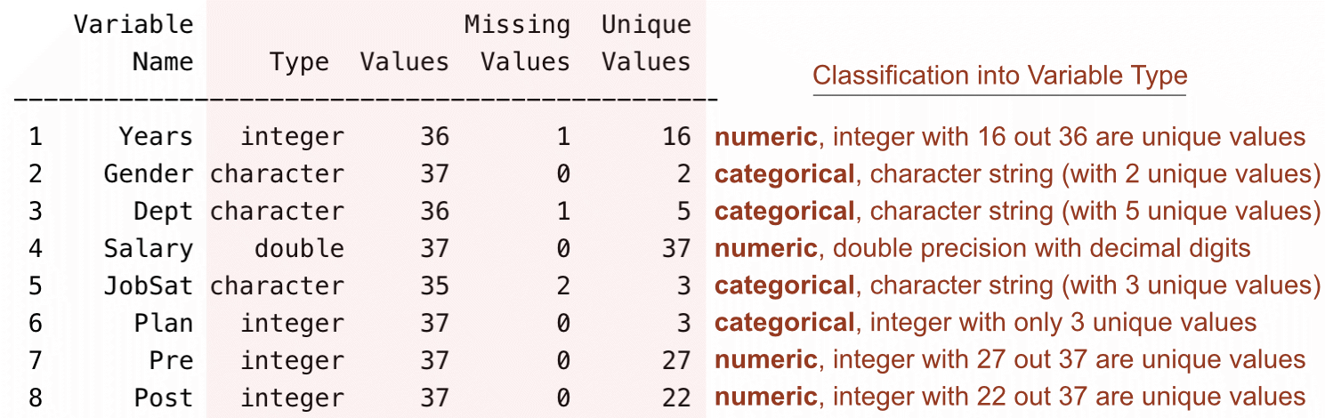
lessR function details().We can identify the categorical variables by examining the type of variable as read into the system and then comparing the number of unique values to the number of values. We can also verify that the numeric variables have been assigned the correct variable type.
Formal Categorical Variables
Regardless of whether categorical variables are read into the data analysis app as integers or character strings, a special data type for categorical variables is typically required beyond the variable type by which the data were read.
The issue is that reading the data into any data analysis app, such as R or Python, requires more information to analyze the categorical variables than the data provides.
Three general issues for categorical variables typically require answers before data analysis begins.
- For non-numeric data values, properly order the levels, such as Low, Medium, and High
- For integer data values, attach meaningful labels to integer data values
- For either non-numeric or integer levels, display potential response categories that did not occur in the data
Answering these questions requires transforming the original integer or character string data types to a formally defined categorical variable. Here are the variable types for this formal representation, created only by transforming the data as initially read.
- R:
factor - Python:
category
To save memory, variables defined by these formal categorical variables store the categories as integers but display the categories as non-numeric labels.
It is possible to leave categorical variables in their character string or integer form as read into the analysis app. Still, it is almost always preferred to transform each categorical variable as read into the system to a formal categorical variable, either a factor for R or a category variable type for Python. This transformation not only to saves memory but also can provide answers to the three general issues listed above.
Before analysis begins, convert categorical variables, read initially as integers or character strings, to formal, properly defined categorical variables.
Each of the three general issues is addressed in the following sections. But first, we show how to convert a variable to an R factor or a Pandas category type variable where the given levels of the variable are accepted as they exist in the data. With no explicit instructions, the default ordering of levels, which is numerical for integers and alphabetical for character string variables, is also accepted.
Accept Existing Levels
Suppose Gender is assessed with one of three character strings: ‘M’, ‘W’, and ‘O’ for other. The data values sufficiently indicate their meaning. The default alphabetical ordering of the levels can be accepted without modification. In this situation, convert the character string variable as read to a formal categorical variable without the need for specifying additional information.
R
The Base R function factor() converts a variable read from the data as type integer or character to an R factor. As indicated, the values of Gender are character strings. Instead of displaying a description of all the variables with the lessR function db(), here, use the base R function class() to only show the variable type of Gender.
class(d$Gender)[1] "character"Because the levels of Gender in this data set are sufficiently descriptive and the alphabetical ordering of the levels is appropriate, the factor() function can be invoked without specifying any parameter values.
Identify the corresponding data frame when referencing a variable, such as the JobSat variable, so that R can locate the variable. It is possible, for example, to have multiple current data frames, each with a variable called JobSat. Identify the containing data frame by preceding the variable name with the name of the data frame followed by a dollar sign, $.
d$Gender <- factor(d$Gender)
class(d$Gender)
[1] "factor"After the transformation, the variable Gender in the d data frame is now of variable type factor.
Python
To transform Gender in the df data frame to a variable of type category, invoke the astype() function with the parameter value category.
df['Gender'] = df['Gender'].astype('category')
df.dtypes
Years float64
Gender category
Dept object
Salary float64
JobSat object
Plan int64
Pre int64
Post int64
dtype: objectGender is now a variable of type category.
Order Character String Levels
In the Employee data set, three levels describe the categorical variable JobSat: low, med, and high. From this data, construct the bar chart, here from the lessR function BarChart(), but the same principle applies to Python.
BarChart(JobSat, quiet=TRUE)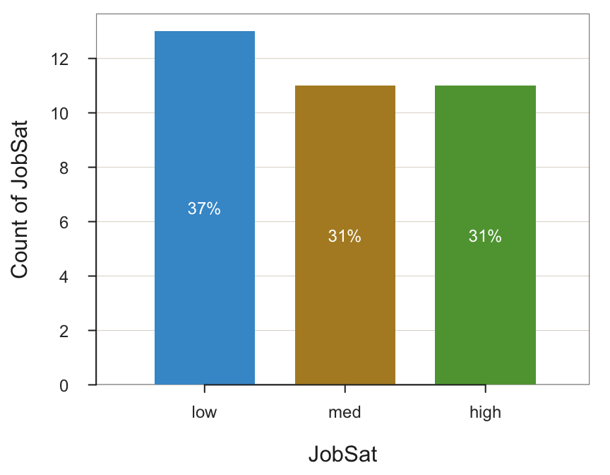
Oops! Neither R nor Python knows the meaning of words such as “low”. They have to choose some arbitrary ordering of the bars, which is an alphabetical ordering by default. Analyses that involve the unmodified JobSat variable present the levels in the wrong order: high, low, and med.
R
To properly order the character string levels of a categorical variable, convert the variable from type character as initially read into R to type factor with the factor() function. To specify the desired order, we need to introduce the levels parameter of the factor() function.
levels parameter for
factor(): Specify the desired ordering of the categorical variable’s levels as they exist, or could exist, in the data.
Replace the current JobSat variable with its factor version. List the levels in the desired order, what can be called their presentation order in subsequent visualizations.
d$JobSat <- factor(d$JobSat, levels=c("low", "med", "high"))Now that JobSat is of type factor, the bar chart is properly displayed, with the bars in the correct order.
BarChart(JobSat, quiet=TRUE)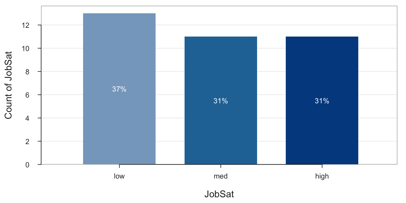
Once converted, there is no need for the original character version of JobSat, so the preceding transformation replaced the original with the factor version. Or, create a new variable in the d frame by entering a new variable name in the left-hand side of the specification before the <-.
The optional ordered parameter for factor() indicates that the levels progress in magnitude from “less” to “more”. Ordering the levels with the levels parameter specifies their display order. Setting the ordered parameter to TRUE goes further than specifying the presentation order to indicate that the factor variable is an ordinal variable. By default, the value of ordered is FALSE, which indicates a nominal variable. For subsequent data visualizations, ordered factors have different default color palettes than non-ordered factors that reflect the underlying ordering.
When the levels of a factor are ordered, the BarChart() color default progresses from light to dark colors, all sharing the same hue. The gradation in lightness reflects the gradation in the ordered values of an ordinal variable.
d$JobSat <- factor(d$JobSat, levels=c("low", "med", "high"), ordered=TRUE)
BarChart(JobSat, quiet=TRUE)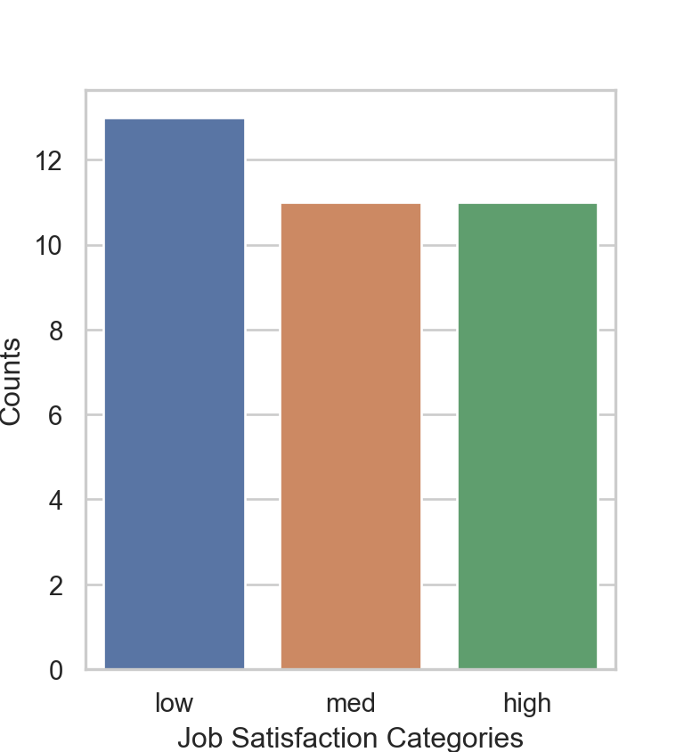
In this example, the levels of the categorical variable were retained, only their order changed. However, the existing levels also could be relabeled, for example, “med” to “medium” in the subsequent output of data analysis functions. This relabeling is pursued in a subsequent section, in the context of assigning labels to integer values of a categorical variable.
Python
Convert the JobSat column to a categorical variable with ordered categories. Invoke the Pandas function CategoricalDtype() to specify the categories and then the astype() function to implement the ordering.
JobSat_cat = pd.CategoricalDtype(categories=['low', 'med', 'high'], ordered=True)

df['JobSat'] = df['JobSat'].astype(JobSat_cat)
df.dtypes
Years float64
Gender category
Dept object
Salary float64
JobSat category
Plan int64
Pre int64
Post int64
dtype: objectPlot a bar chart of JobSat with seaborn, referred to by its abbreviation sns. Invoke the function countplot(). Some analysts still use the older matplotlib for visualizations, but seaborn is easier and produces more aesthetic visualizations.
sns.set(style="whitegrid")

plt.figure(figsize=(4, 4.4))
sns.countplot(x='JobSat', data=df)

plt.xlabel('Job Satisfaction Categories')
plt.ylabel('Counts')
plt.show()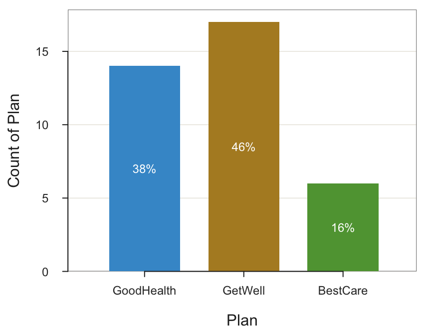
The bars are now listed in the correct order by converting JobSat to a variable of type category with the proper order specified.
Label Integer Values
The levels of a categorical variable may be coded as integers. For example, for the employee data, the variable Plan is categorical, coded in the data file with the integers 1, 2, and 3 corresponding to three health plans, respectively named GoodHealth, GetWell, and BestCare. The corresponding bar graph necessarily displays these integer values, here illustrated in R/lessR.
BarChart(Plan, quiet=TRUE)
The resulting visualizations are more meaningful with the output labeled with the names instead of integers, so transform a categorical variable read into a data frame as integers into a formal categorical variable with the corresponding labels.
R
To assign integer values, follow the same general procedure as the previous example that transforms a variable of type character into a factor but also introduces the labels parameter to provide more meaningful value labels. The data values are integers, 1 through 3, so the levels parameter has the corresponding integer values, the integer vector 1:3, an abbreviation for c(1,2,3).
labels parameter of
factor(): The value labels to attach to the levels in the data frame for the corresponding categorical variable.
In the following function call to factor(), the labels parameter is written underneath the levels parameter to help ensure that the labels match the levels in the desired order.
d$Plan <- factor(d$Plan, levels=1:3,
                         labels=c("GoodHealth", "GetWell", "BestCare"))
Verify that the variable type of Plan has changed from integer to a factor.
class(d$Plan)[1] "factor"This revised bar chart contains the more descriptive labels in place of the original integers.
BarChart(Plan, xlab="Health Plan Categories", quiet=TRUE)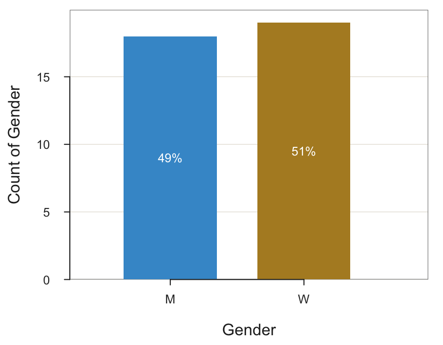
This example ordered the levels in the sequence of 1, 2, and 3 because the levels were listed in that order defined by the vector 1:3. Other vectors could have been entered, such as c(3,1,2), to specify a different order. Regardless of the specified order of the levels, the ordering of the labels must match the exact ordering so that each label matches its corresponding level.
The labels applied in this example are attached to integers. The labels parameter can also apply to variables of type of character. In that situation, display the original character as levels with another set of labels. For example, for the categorical variable Gender, display on the output a data value of "M" with the value label "Man".
Python
Character string variables are initially read as variable type object. Without missing data, integers are read as type integer. However, for Pandas to keep things a little complicated, if there are missing values, NaN, Pandas reads the non-missing integers as a float data type because the standard integer type does not support missing data.
In the Employee data, convert the type int64 variable ‘Plan’, for health plan, to type category with labels ‘GoodHealth’, ‘GetWell’, and ‘BestCare’ for 1, 2, and 3, respectively. This conversion requires two steps. First, define a Python dictionary with the assignment from integers to character strings. Then, implement the change with the map function followed by astype() to do the conversion to type category.
Plan_map = {1: 'GoodHealth', 2: 'GetWell', 3: 'BestCare'}
df['Plan'] = df['Plan'].map(Plan_map).astype('category')
Display the first few rows of the data frame to verify the changes.
df.head() Years Gender Dept Salary JobSat Plan Pre Post
Name
Ritchie, Darnell 7.0 M ADMN 53788.26 med GoodHealth 82 92
Wu, James NaN M SALE 94494.58 low GoodHealth 62 74
Downs, Deborah 7.0 W FINC 57139.90 high GetWell 90 86
Hoang, Binh 15.0 M SALE 111074.86 low BestCare 96 97
Jones, Alissa 5.0 W NaN 53772.58 NaN GoodHealth 65 62Show the variable types.
df.dtypesYears float64
Gender category
Dept object
Salary float64
JobSat category
Plan category
Pre int64
Post int64
dtype: objectWith the transformation of Plan to type category and the assignment of the corresponding value labels, the resulting bar chart is now more descriptive.
sns.set(style="whitegrid")

plt.figure(figsize=(4, 4.4))
sns.countplot(x='Plan', data=df)

plt.xlabel('Health Plan Categories')
plt.ylabel('Counts')
plt.show()
Plan is not a variable that stores the assigned labels as if it contained those character strings as data values. Because Plan is a variable of type category, these labels do not require the memory that would be needed if they were character strings. Instead, the data of a category variable are saved as integers.
Add Levels Beyond the Data
Sometimes, not all possible responses for a categorical variable occur for one or more variables. The resulting visualization should usually include an analysis of potential responses, including those for categories with zero response. To do so, the visualization procedures must be made aware of potential data values that do not exist in the data.
R
We have modified Gender from the original data table, so re-read.
d <- Read("Employee", quiet=TRUE)Invoking the lessR function pivot() generates the following frequency table for Gender of the data unmodified as read into the R d data frame.
pivot(d, table, Gender) Gender Freq Prop
1 M 18 0.486
2 W 19 0.514The possible values for Gender are M, W, and O for other. However, in this small data set there were no responses for O, so the frequency table and corresponding bar chart cannot show a count of 0 for this category as it does not exist in the data. Fortunately, factor() allows the inclusion of all possible data values, not just those that occurred, as shown here. Simply define all possible levels of the categorical variable, and here also provide the optional labels for greater clarification of the meaning of each level.
d$Gender <- factor(d$Gender,
                   levels=c("M", "W", "O"),
                   labels=c("Man", "Woman", "Other"))
Now that O as a level with corresponding label Other is defined, the value of Other is included in analysis output even though never occurring in the data.
BarChart(Gender, quiet=TRUE)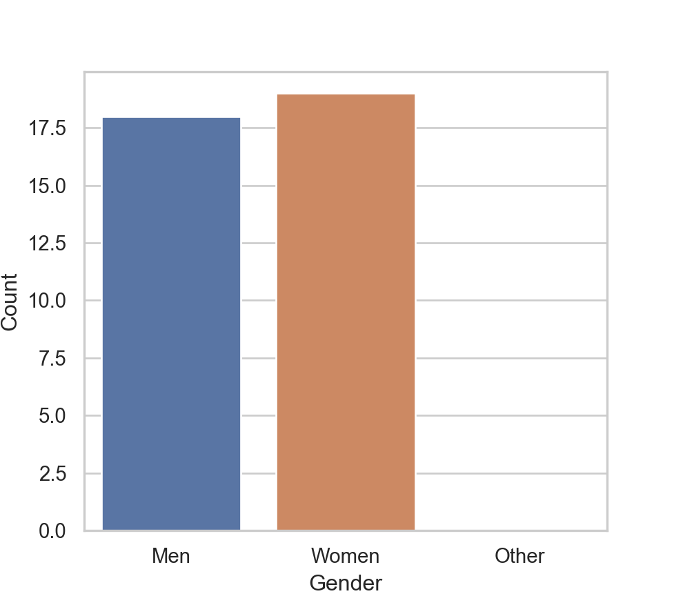
Python
Compared to R, transforming Gender to the category variable type with values that do not occur in the data has no effect here. The map() function only maps according to the actual data values in the data table. Here, convert to a type category variable to provide the Men and Women labels without wasting memory. The conversion itself is not necessary to obtain the bar chart.
Gender_map = {'M': 'Men', 'W': 'Women'}
df['Gender'] = df['Gender'].map(Gender_map).astype('category')
To show the bar chart with a potential data value with 0 count in this data set requires manually constructing the table of frequencies from which the bar chart will be constructed, instead of from the original data.
Gender_freq = df['Gender'].value_counts()
print(Gender_freq)
Gender
Women 19
Men 18
Name: count, dtype: int64Once the table of counts of the Gender existing values is obtained with value_counts(), manually add another label, here ‘Other’ with a count of 0.
if 'O' not in Gender_freq:
    Gender_freq['Other'] = 0
Reset the row index to have Gender as a variable instead of the row name, the index. Then name the variables as Gender and Count.
Gender_freq = Gender_freq.reset_index()
Gender_freq.columns = ['Gender', 'Count']
print(Gender_freq)
Gender Count
0 Women 19
1 Men 18
2 Other 0Create the plot from this revised table of counts, now using the barplot() function instead of the previously used countplot(). The distinction is that for countplot(), you pass a single categorical variable to the function and it then plots the counts on the y-axis based on the original data frame. For barplot(), you are working from a summary table and so pass the categorical variable as well as the corresponding customized y-value, which can be anything. In this example, the y-axis represents counts but now read directly from the summary table.
plt.figure(figsize=(5.1, 4.5))
sns.barplot(x='Gender', y='Count', data=Gender_freq,
            order=['Men', 'Women', 'Other'])
plt.xlabel('Gender')
plt.ylabel('Count')
This procedure for accounting for non-occurring data values works but is bulkier than the corresponding R and lessR implementation, requiring only two lines of code to produce the bar chart. Moreover, because the Pandas category variable type does not store unused categories, the desired order of the levels must be specified for every analysis, such as the corresponding bar graph.