The Concept
Data consists of data values.
Examples of data values include:
- A person’s height.
- The GNP of a country.
- The cost of a gallon of milk at the local grocery store.
- A shipment delivery time.
Refer to the data for each person, unit, or object with one of many possibilities, including observation, example, instance, sample, and case.
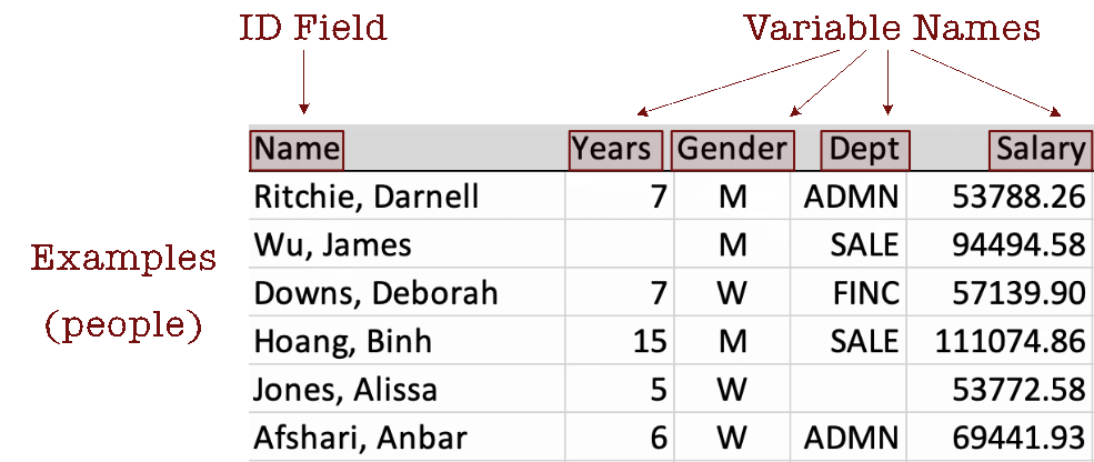
Organize data values into a table, such as the following example. Each row contains the data values for a specific observation, here an employee. Data values for an observation are provided across the variables in the data table as a row of data values. Each column contains the data values for a given variable, providing that all data values within a column have the same format.
Store the data table in a computer file, constructed in various ways, ranging from automated systems to manual data entry into Excel. This computer file exists independently of any application, such as R or Python from which the data will be analyzed. Regardless of how the original computer file was obtained, it must be read into R or Python, or whatever, for analysis.
For analysis, convert the stored data table into a data structure that exists within the running data analysis application, such as R or Python. In Excel, store the data table in a worksheet. An Excel worksheet that stores a data table, when represented within R or Python, is called a data frame.
The concept of a data frame is an essential data analysis concept.
Virtually all data analysis is of variables stored in a data frame, constructed from data read from an external data table stored as a computer file in a specified format.
The formats for the data file vary from Excel to text files to specialized file formats optimized for big data, a topic covered in another reading.
Two Data Frames
A primary characteristic of a data frame is consistency. All data values for a variable must be stored within a single column in a consistent format. The meaning of this consistency is explored in the following two representations of a data table, one illustrating inconsistency that would not be amenable to analysis and one table properly, consistently formatted.
The Bad
Unfortunately, data tables typically do not arrive ready for analysis. Here is an example of a very poorly formatted data table in Excel.
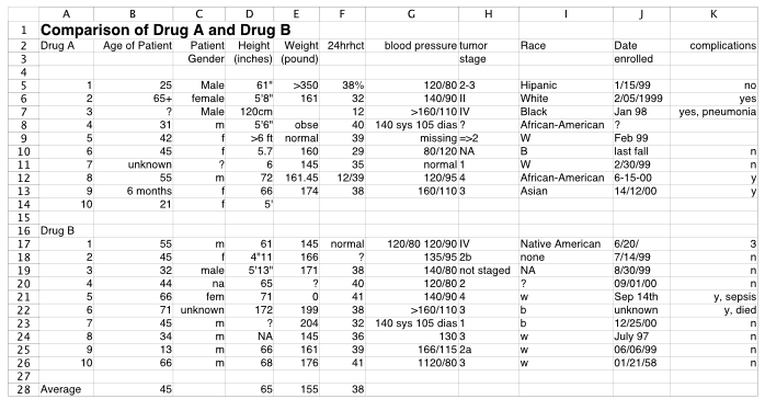
The preceding table would require much work before the data could be read into a data frame amenable to analysis. So many problems describe this table.
- Text appears in columns of numerical variables, such as 65+ for Age,
Cell B6. - The same category for categorical variables is coded differently for different people, such as “Male”, “male”, and “m” for male,
Column C. - Missing data coding is inconsistent, such as “unknown”, “?”, blank cell, and “NA”,
Cells B11, C11, K8, D24. - One variable, “complications” is a combination of two variables, a binary “yes” or “no”, and then a description of the complication if there is one,
Column K. - Drug is a variable, with two values, A and B, yet the data for the two drugs are presented in two different data tables, both within the same worksheet,
Column A. - The first line of the data table should be the variable names. The title of the project belongs in the corresponding code book to describe the contents of the data file, which can be stored in a separate file or a second worksheet after the data,
Row 1. - The data table includes statistical calculations, averages of some columns, beyond just data,
Row 28. - Dates are expressed in different date formats,
Column J. - Some variable names take up two columns instead of a single name in a single cell in the first row of the data table,
Cells C3, C4.
The Good
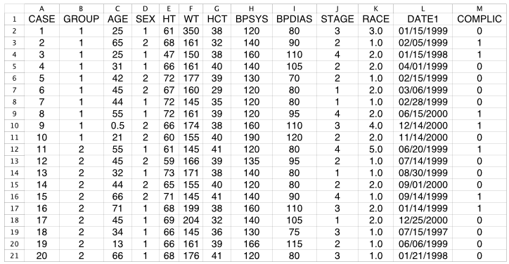
Following is a well-formatted data table, ready to read into R, Python, or virtually any data analysis app to begin analysis. The only potential issue is that all coding is numerical, even for categorical variables, which, by definition, are non-numerical. For example, the two different drugs are labeled as Drug A and Drug B, yet they are coded with values of 1 and 2 under a variable named Group.
Even if the values of a categorical variable are represented with integers, the data values have no numerical meaning; they are just labels. Fortunately, integer coding of categorical variables is not much of an issue if a proper code book accompanies the data table. In that case, attach the value labels to the integer codes by converting the integer variable to a formal categorical variable of type factor in R or of type category in Python Pandas.
A common understanding in the data science industry is that data preparation and cleaning to prepare the data for analysis typically accounts for 75% to 85% of the required total project time. Of course, this problem is more acute with manually entered data, though there is no guarantee that just because a data entry process is automated a clean data table results.
Understand Your Data
When reading the data into a data frame, you should understand the properties of the data values for the variables read before the analysis begins.
Your data file’s contents are a different representation of your data as stored in a data frame, which may or may not correspond to your view of how your data resides in the data frame.
All analysis depends on accurately referring to the variable names, including the pattern of capitalization, yet even something as basic as the variable name can change from the way the name is listed in the data file and the way it is represented in the data frame. For example, in R any spaces in a variable name in the data file are converted to periods when read into an R data frame.
Other considerations concern the amount of missing data and classifying the variables as continuous or categorical, discussed in detail elsewhere. Or, if you are reading data from a .csv file and the data values for the variable Salary contain \$ signs or commas, then the data are read as character strings instead of numbers. Information regarding these issues should be obtained and evaluated before analysis begins.
R
Access lessR.
suppressMessages(library(lessR))Read the data set Employee, an internal data set downloaded with lessR. This information should always be reviewed before proceeding with an analysis of that data.
d <- Read("Employee")Data Types
------------------------------------------------------------
character: Non-numeric data values
integer: Numeric data values, integers only
double: Numeric data values with decimal digits
------------------------------------------------------------
Variable Missing Unique
Name Type Values Values Values First and last values
------------------------------------------------------------------------------------------
1 Years integer 36 1 16 7 NA 7 ... 1 2 10
2 Gender character 37 0 2 M M W ... W W M
3 Dept character 36 1 5 ADMN SALE FINC ... MKTG SALE FINC
4 Salary double 37 0 37 53788.26 94494.58 ... 56508.32 57562.36
5 JobSat character 35 2 3 med low high ... high low high
6 Plan integer 37 0 3 1 1 2 ... 2 2 1
7 Pre integer 37 0 27 82 62 90 ... 83 59 80
8 Post integer 37 0 22 92 74 86 ... 90 71 87
------------------------------------------------------------------------------------------To facilitate this understanding, when reading data, the lessR function Read() reports the name of each variable, the data storage type of each variable, the number of non-missing values, the number of unique values, and provides sample data values. Obtain this analysis of the variables in a given data frame at any time during an R analysis with the lessR function details_brief(), abbreviated db(), with the name of the data frame as the first parameter value. By default, Read() calls db() after the data are read. Turn off the report by setting the quiet parameter to TRUE.
Obtain more information regarding missing data values by asking for the full report, calling the full details() function. Set the parameter brief to FALSE for more information.
d <- Read("Employee", brief=FALSE)
----------------------------------------------------------
Dimensions: 8 variables over 37 rows of data
First two row names: Ritchie, Darnell Wu, James
Last two row names: Anastasiou, Crystal Cassinelli, Anastis
----------------------------------------------------------
Data Types
------------------------------------------------------------
character: Non-numeric data values
integer: Numeric data values, integers only
double: Numeric data values with decimal digits
------------------------------------------------------------

    Variable                  Missing  Unique
        Name     Type  Values  Values  Values   First and last values
------------------------------------------------------------------------------------------
 1     Years   integer     36       1      16   7  NA  7 ... 1  2  10
 2    Gender character     37       0       2   M  M  W ... W  W  M
 3      Dept character     36       1       5   ADMN  SALE  FINC ... MKTG  SALE  FINC
 4    Salary    double     37       0      37   53788.26  94494.58 ... 56508.32  57562.36
 5    JobSat character     35       2       3   med  low  high ... high  low  high
 6      Plan   integer     37       0       3   1  1  2 ... 2  2  1
 7       Pre   integer     37       0      27   82  62  90 ... 83  59  80
 8      Post   integer     37       0      22   92  74  86 ... 90  71  87
------------------------------------------------------------------------------------------
Missing Data Analysis
------------------------------------------------------------
Number of cells in the data table: 296
Number of missing data values: 4
Proportion of missing data values: 0.014
Number of rows of data with missing values: 3
------------------------------------------------------------
Years Gender Dept Salary JobSat Plan Pre Post
Wu, James NA M SALE 94494.58 low 1 62 74
Jones, Alissa 5 W <NA> 53772.58 <NA> 1 65 62
Korhalkar, Jessica 2 W ACCT 72502.50 <NA> 2 74 87
------------------------------------------------------------With this more detailed report, we can see how much missing data is found in each row of the data table and what proportion of all the data values are missing. By default, only 30 rows with missing data are displayed to minimize the size of the output for large data sets. Customize this value with the miss_show parameter by setting its value to any arbitrary number. Or, further customize the output with the n_mcut parameter that specifies the minimum number of missing data values in a row before displaying that row. The default value is 1, but again, can be set to any arbitrary value.
Getting rid of missing data is easy. To remove all rows of data (cases) that contain at least one missing value, use the Base R na.omit() function.
nrow(d)[1] 37d <- na.omit(d)
nrow(d)[1] 34Three rows of data have been deleted from the d data frame, the three rows with missing data.
Python
Access pandas, numpy upon which pandas depends, and the standard visualization packages.
import pandas as pd
import numpy as np
import matplotlib.pyplot as plt
import seaborn as sns
Read the Employee data from the web into the df data frame. The first column, Column 0, consists of the unique ID’s that identify each row, the employee’s name. Setting parameter index_col to 0 sets the contents of that columns to row names in the subsequent data frame.
df = pd.read_excel("~/Documents/BookNew/data/Employee/employee.xlsx",
                   index_col=0)
To understand the data that was read into a Pandas data frame, perform the following operations for the df data frame that returns a result for each variable in the data frame.
- variable type with
df.types - count of non-missing data values with
df.count() - count of the number of missing values with
df.isna().sum() - count of the number of unique values with
df.nunique()
For a convenient display of properties of your data, concatenate the resulting four vectors (each a Python series) into a data frame with the Pandas function concat() for concatenation. Then, change the default column names, the consecutive integers beginning with 0, to meaningful names with the concat() parameter keys.
Define a function, details(), that implements these operations for easy cutting and pasting to other Python programs. Provide the option with the brief parameter that, when set to False, displays all rows of data that contain missing data. The default value of brief is True, so unless specified, the rows with missing data are not displayed. Pandas must have been imported before the function is called.
# d is the data frame parameter
def details(d, brief=True):

    ty = d.dtypes
    nv = d.count()
    nm = d.isna().sum()
    nu = d.nunique()
    dStats = pd.concat([ty,nv,nm,nu], axis='columns',
                       keys=['type', 'values', 'missing', 'unique'])
    print(dStats)

    if not brief:
      print("\n")
      print(df[df.isna().any(axis='columns')])
Call this details() function with the current data frame, df. Set brief to False to also obtain the rows of data with missing values.
details(df, False) type values missing unique
Years float64 36 1 16
Gender object 37 0 2
Dept object 36 1 5
Salary float64 37 0 37
JobSat object 35 2 3
Plan int64 37 0 3
Pre int64 37 0 27
Post int64 37 0 22
Years Gender Dept Salary JobSat Plan Pre Post
Name
Wu, James NaN M SALE 94494.58 low 1 62 74
Jones, Alissa 5.0 W NaN 53772.58 NaN 1 65 62
Korhalkar, Jessica 2.0 W ACCT 72502.50 NaN 2 74 87Without creating my own Python package to run the above code and elaborate on this code, copy and paste this function at the beginning of every analysis after the data is read. Again, always understand your data before you begin to analyze that data.
The code for viewing all rows of missing data begins with the Pandas function isna(), which returns True if a data value is missing. The any() function evaluates the data frame column-by-column and then returns True if there are any True values in the corresponding row. Putting the expression within d[ ] selects only the rows with True, that is, with missing according to isna(). Find more information regarding then df[ ] notation in the material that describes data wrangling.
Getting rid of missing data is easy. To remove the all rows of data (cases) that contain at least one missing value, use the Pandas drop.na() function.
df.shape(37, 8)df = df.dropna()
df.shape(34, 8)We see that three rows of data have been deleted from the df data frame, the three rows with missing data.