Introduction
Data easily flows in and out of all the primary data analysis languages because they easily read and write data from and to standard data file formats shared by all major data analysis languages.
If the data file is saved in a widely-recognized storage format, analyses can proceed from any data analysis system that recognizes that format. As we will see, the cross-platform formats are typically the best in terms of speed and efficiency.
Data exists within an executing analysis program as a data frame. That data frame is the internal representation of the data as a standard data table, typically read from an external computer file into the data frame. Data exists stored as a computer file independently of any data analysis system, then read into the data analysis system represented as a data frame. If needed after any data transformations and manipulation within the analysis system, the revised data can be written again to a new data file or over the existing data file.
The syntax for a particular operation in a specific language need not be memorized and can always be recovered from the web. As always, what is important is to understand are the concepts. Data exists in an external file, which can be according to one of the multiple formats, and that the data can enter and leave any analysis system easily with straightforward function calls to read and write data from and to external files.
A reference to a Web URL or a path name on your computer system to identify the location of a data file is a character string constant, and so is enclosed within quotes. The use of double or single quotes is an arbitrary choice for R or Python, though the tradition is to typically use the double quotes in R and the single quotes in Python. Working with variables in Python typically requires including each variable name in quotes, while R typically allows variable names to be written free of quotations.
The analysis of data begins with one or more data files from some source. When the analyst receives that data file, the first step is to set it to Read Only.
One common mistake is for an analyst to receive an Excel data file, and then immediately start cleaning and transforming the data. Problem #1 is that any errors are not recoverable. Problem #2 is the difficulty documenting changes made to the data.
Instead of changing the original data, the Read Only status of the original data file specifies no changes to that file. Instead, the cleaning and data transformation occurs as a result of code, such as R or Python code files, that indicate a specific set of changes made to the original data to prepare the data for analysis. These changes can always be repeated with an needed modifications given that the original data remain unchanged and the changes are documented. Once transformed and prepared, then, following the instructions below, write the data to an data file for everyone on the team to access for the analyses.
Text Data Files
Two of the most commonly encountered data file formats are csv for comma separated values text files and Excel. Both formats work well for small to perhaps medium size data files, but are much more inefficient in terms of storage and I/O speed than modern data file formats. Reading and writing large data files will take relatively much longer with these formats than with available alternatives.
The primary text file formats are csv for comma separated file and tsv for tab separated file.
Excel files in the xlsx format are also text files, though organized in an open, public, though Microsoft defined format, a version of the open standard, text-based XML called Open XML. Neither R nor Python, as initially provided, read Excel data files, so each requires an external package.
Microsoft was forced to move to an open document format in 2007. The EU and many individual European governments, such as Germany, France, and the UK, would no longer store documents in a binary format that only Microsoft could decode. Thus, the move from .doc to .docx, .xls to .xlsx, etc., or these governments would have likely switched to the capable free, office suite with an open document format, LibreOffice (then called Open Office). Even so, hundreds of thousands of European government computers now run LibreOffice instead of MS Office.
Realize, however, that writing data to a text file can lose the unique variable storage formats provided by an analysis system. All data values in a text file are represented as a character string. Reading text into a data frame requires the computer to identify, for example, which character strings represent numbers and then internally transform those characters into numeric values.
Writing text requires that unique properties attributed to the data values are lost because all that remains are simple character strings. For example, after reading text data into an analysis system, all categorical variables should be explicitly and manually defined as such, factor or category variables in R and Python, respectively. These definitions are lost when the data are written as text to a csv, tsv, or Excel file.
R
Unlike Python, R does not require listing the package name (or abbreviation) with each corresponding function call, though for clarity the name can included with the use of double colons, ::, such as lessR::Read(""). Including the package name is recommended when using functions from different packages, particularly for code that you intend to share with colleagues. Of course, each external package from which functions are accessed in your code must first be retrieved from the R library with the library() function.
Unlike any other function of which I am aware in any data processing system, my lessR function Read() does not require you to specify the specific read function for a specific file format. Instead, Read() learns the format, by default, from the file type, such as .xlsx for Excel files. After determining the file type, Read() automatically selects the proper read function to match the file format of the data, and can read many formats. For example, Read() implicitly relies upon:
- the Excel read and write functions provided by the
openxlsxpackage to process reading Excel data - the Base R functions
read.csv()andwrite.csv()to read or write acsvdata file - functions from the
readODSpackage to read files in the LibreOffice worksheet format - and many others
You can override this default with the format parameter if, for some bizarre reason, you decide to use a non-standard file type.
Another unique feature of Read() is that if you do not specify a web URL or path name between the quotes, then you are instructing R to browse for the file on your computer system. Once located, the data are read into the specified data frame, and the full path name is then displayed in the R console so you can copy and paste it for future reference, allowing you to directly read the data file.
Read() can also read csv or tsv files without any additional specification. The function automatically detects if adjacent data values are separated with a comma or with a tab.
library(lessR)
d <- Read("http://lessRstats.com/data/employee.xlsx")
d <- Read("http://lessRstats.com/data/employee.csv")
See the manual for more documentation by entering ?Read into the R console, and the vignette that provides multiple examples with documentation, either from entering browseVignettes("lessR") into the R console or on the web. For example, unlike other systems, lessR provides for variable labels, also read by Read() according to the var_labels parameter. Missing data can be identified, such as if codes such as -99 are used to identify missing data, and a specified number of lines can be skipped before reading from a text or Excel file.
Also, unlike any other read function in R or Python of which I am aware, Read() also provides helpful information regarding the information read into a data frame, such as the number of unique data values for each variable to assist in identifying categorical variables. Other parameters, such as miss_show, provide even more information regarding missing data in your data table.
Complete the I/O operations with the lessR function Write(), illustrated below, for writing the contents of the data frame d to an Excel or csv file format.
Write(d, "employee", format="Excel")
Write(d, "employee", format="csv")
If writing to an Excel file, set the ExcelTable parameter to TRUE to write the data as an Excel Table instead of the default worksheet format.
Python
Python uses the import method to play the same role as the R library() function. Python allows an abbreviation to represent the package, i.e., module name. The primary data manipulation package of functions in Python is pandas, usually abbreviated pd. Indicate that a specific function is sourced from a specific add-on package with the package name or abbreviation followed by a period before the function name.
Read these files with the read_excel() or read_csv() functions.
import pandas as pd
d = pd.read_excel('http://lessRstats.com/data/employee.xlsx')
d = pd.read_csv('http://lessRstats.com/data/employee.csv')
Write Excel or csv files with the to_excel() or the to_csv functions.
d.to_excel('employee.xlsx')
d.to_csv('employee.csv')
It is easy to provide the data in Excel format to those colleagues whose data skills are limited to Excel.
Binary Data Files
For large data files, best to write and then read in a binary format.
Binary file formats are designed to be more efficient for I/O than text-based files, typically requiring less storage space and providing much faster I/O. Common examples of binary files are executable files, image files, audio files, and video files. Add many data files to that list.
Besides efficiency, binary files can also offer the advantage of saving data exactly as it exists within a data frame. For example, categorical variables formally defined as an R factor or Pandas category variable type will remain so defined in the corresponding binary file of that data frame written to a data file.
Native R Binary File
R has its own native, binary format, directed primarily for exclusive R work1. Base R defines functions save() and load() to write and read R native format files, but lessR simplifies this process in pursuit of the goal of minimizing the number of functions needed for data analysis. Instead, the usual lessR functions Read() and Write() read and write binary R files the same way other file formats are read and written. Indicate a binary R file with the format parameter set equal to R.
1 A Python package (module) is available to read binary, native format R files directly, pyreadr.
Write(d, "employee", format="R")
d <- Read("employee", format="R")
Parquet and Feather
Feather and parquet are fast, lightweight, and easy-to-use, recommended binary file formats for storing data tables. Both formats are based on Apache Arrow, and so serve as an excellent basis for data interchange between R and Python. Version 1 of feather was initially designed by Hadley Wickham of RStudio fame, and author of many R packages such as ggplot2 and dplyr, and Wes McKinney, the creator of Pandas. The appearance of the second version of feather in 2019 greatly enhanced the format. Both feather and parquet are excellent, modern file formats. Both formats produce relatively smaller data file sizes and excellent performance.
R
Feather and parquet are available within R as part of the functionality of the arrow package. As with any external package, first, download the package from the R servers with the install.packages() function.
install.packages("arrow")feather
Once the arrow package is accessed, writing and reading the feather format and straightforward with the functions write_feather() and read_feather(). The default parameter value of parameter version for write_feather() is 2, which is the only version to access unless reading legacy data. Here, write the d data frame to a feather file and then read back into the d data frame with read_feather().
library(arrow)
write_feather(d, "employee.feather")
d <- read_feather("employee.feather")
Or, from lessR Version 4.3.1 onward, proceed with the usual Write() and Read() functions, with no need for library(arrow) as that will be handled internally by lessR.
Write(d, "employee", format="feather")
d <- Read("employee")
parquet
Once the arrow package is accessed, writing and reading the parquet format is straightforward with the functions write_parquet() and read_parquet(). Here, write the d data frame to a parquet file and then read it back into the d data frame.
library(arrow)
write_parquet(d, "employee.parquet")
d <- read_parquet("employee")
Or, from lessR Version 4.3.1 onward, proceed with the usual Write() and Read() functions, with no need for library(arrow) as that will be handled internally by lessR.
Write(d, "employee", format="parquet")
d <- Read("employee")
Pandas
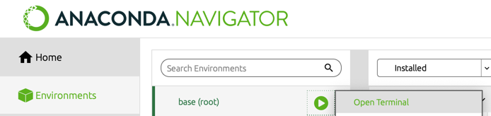
Accessing feather and parquet from within Python requires the pyarrow package (module), which works with Pandas. With the Anaconda Python distribution, this package may need to be separately installed. From the command line, such as the Macintosh Terminal app, enter the following.
conda install pyarrowOne way to access the command line is from within Anaconda Navigator as shown here.
feather
With pyarrow downloaded and installed, here write the d data frame to a feather file. The default version parameter is 2 for Version 2 of feather. Do the writing with the to_feather() function and reading with read_feather().
import pandas as pd
d.to_feather('employee.feather')
d = pd.read_feather('employee.feather')
parquet
Here, for the d data frame, do the writing with the to_parquet() function and reading with read_parquet().
import pandas as pd
d.to_parquet('example.parquet')
d = read_parquet("example.parquet")
Evaluate the File Formats
How efficient are the various file formats in terms of speed and file size? Tests were run on a reasonably large set of data to evaluate the different possibilities.
Example Data
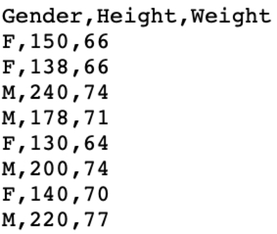
To illustrate the relative speed and size of reading data files in the various data file formats, using the R random normal number generator, rnorm(), I constructed a relatively large data frame of 100,000 records. The data frame contains these ten numerical variables with 15 significant digits each and also five Yes/No categorical variables. Following are the first three rows of the data frame. To show all the digits with head(n=3), the default number of displayed significant digits was increased from 7 to 15 with the R function parameter(digits=15).
                  X1   ...                 X10 Xcat1 Xcat2 Xcat3 Xcat4 Xcat5
1  1.419335043355753   ...   1.333228464493326   Yes    No   Yes    No    No
2 -2.439084062984318   ...  -0.744485250085974   Yes   Yes    No   Yes    No
3  0.509216177972103   ...  -0.927332667145959   Yes   Yes   Yes    No    No
This data frame was written in .csv, Excel, native R file formats with the file type .rda for R data file, and feather and parquet formats. Two different Excel functions were evaluated, one from the openxlsx package and one from the readxl package. Also evaluated was the identification of the variable type as part of the read statement, using the col_types parameter from readxl and the colClasses parameter from the Base R read.csv() function.
d <- read.csv(“large.csv”, colClasses=c(rep(“double”, 10), rep(“character”, 5)))
Evaluation
I conducted the speed tests on my M1 Mac Studio Desktop with the function microbenchmark(), from the package of the same name. Each data file was successively read 100 times under each condition to account for random differences in the read times. The results in the following table show the mean read times in seconds for each read function and its respective file size. Of course, realize that these results apply to the specific data file that is being evaluated but do not generalize exactly the same to all data files.
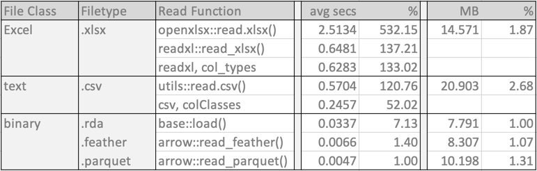
The name before each :: indicates the package in which the function is located. The R packages utils and base are both included in Base R.
The three binary formats are the clear winners in both performance and file size. The binary file formats also offer the advantage of copying all aspects of the data frame as it exists in R. After reading the data, all categorical variables, integer or character string, should be converted to variable type factor for R and category for Python. Saving the updated data frame in a binary format saves these subsequent modifications of the data values. The alternative re-reads the initial text file with the need to re-do the transformations.
Of the binary formats, by far the fastest read times were achieved for the feather and parquet formats. The native R format required a read time of more than seven times longer than the parquet file. Regarding file format size, the native R data file is the smallest. The feather file format is 7% larger, and the parquet format is 31% larger.
The Excel and csv formatted read times were considerably larger. The fastest Excel read time is more than 133 times longer than the for parquet. And their file sizes were also considerably larger, the Excel file 1.87 times larger than the native R file, and the csv data file 2.68 times larger.
If data are already in the csv format, reduce the read time of the csv file by pre-specifying the variable types so that the read function does not need to do the deciphering. This pre-specification allows the read function to read the data directly instead of needing to decipher the storage type for each column. Create a vector corresponding to the variables in the data file that lists each variable type. Example variable types: "integer", "numeric" or"double", and"character" for the read.csv() parameter ColClasses. In this example, the mean read speed decreased from 0.5704 secs to 0.2457 secs, a decrease of more than half. However, this faster read speed is still considerably longer than for the binary formats, and any data transformations to different variable types, such as conversion to factor variables, will be lost. See?read.csv for more information. Because the lessR function Read() relies upon read.csv() to read text files, colClasses is also available for Read().
Conclusion
The results of these analyses are straightforward.
Conclusion: The newer
featherandparquetdata file formats are generally preferred, though their relative advantages are minor for small data sets.
The relative advantages of the binary formats over the Excel and text file formats realized here become magnified when working with true big data. The hundred thousand rows of data in this data file that was analyzed in this example comprises a large data file but not nearly as large as can be found in many analyses in the time of Big Data, which can scale to millions of rows (records) of data.
Of course, if large enough, all of the data file cannot simultaneously fit into memory. One solution to this problem is to only read into the analysis system the subset of variables that will be analyzed. Another solution is to obtain more memory, which becomes more feasible by moving the analysis to the cloud. Or, move to specialized libraries such as Python’s dask that can perform parallel processing of multiple chunks or subsets of the full data set, distributed processing by analyzing the data across a cluster of computers, and also treat disk storage the same as in-computer memory. R packages that can provide various aspects of this functionality include data.table, sparklyr, bigmemory, and disk.frame.