❝ Prediction is difficult, especially when dealing with the future. ❞

Danish Proverb

The Forecast

The Smoothing Parameter

Exponential smoothing is perhaps the most widely used of the many available time series forecasting methods. Exponential smoothing provides a set of weights for computing a forecast of the value of a variable as a weighted average of what occurred for that variable at previous times, with increasingly diminishing emphasis on more distant previous time periods: What happened two time periods ago has less influence than what happened the last time period.

The exponential smoothing algorithm computes the forecast for the next time period by decreasing the forecasting error from the previous forecast of the current time period.

Self-adjusting forecast

Adjust the next forecast at Time t+1 to compensate for error in the current forecast at Time t.

If the current forecast $\hat Y_t$ is larger than the actual obtained value of $Y_t$, a positive difference, adjust the next forecast $\hat Y_{t+1}$ smaller than the current forecast. On the contrary, if the current forecast $\hat Y_{t}$ is too small, a negative difference, then adjust the next forecast $\hat Y_{t+1}$ upward.

The definition of forecasting error remains the same as with any forecasting situation: The difference between what is and what was forecasted to be.

Forecasting error

At Time t, the difference between the actual value of Y and the forecasted value, $\; Y_t – \hat Y_t$.

The error in any specific forecast consists of two components. One component is any systematic error inherent in the forecast, systematically under-forecasting or over-forecasting the next value of Y. Exponential smoothing is directed to adjust to this type of forecasting error.

The second type of error inherent in any forecast is purely random. Flip a fair coin 10 times and get six heads. Flip the same fair coin another 10 times and get four heads. Why? Random, unpredictable fluctuation. There is no effective adjustment to such variation. Indeed, trying to adjust in reaction to random errors leads to worse forecasting accuracy than doing no adjustments.

As such, there needs to be some way to moderate the adjustment of the forecasting error from the current time period to the next forecast. Specify the extent of self-adjustment from the current forecast to the next forecast with a parameter named $\alpha$ (alpha).

Smoothing parameter $\alpha$

Specifies a proportion of the forecasting error that should be adjusted for the next forecast according to $\alpha(Y_t – \hat Y_t), \quad 0 \leq \alpha \leq 1$.

The adjustment made for the next forecast is some proportion of this forecasting error, a value from 0 to 1. Choose a value less than 1, usually considerably less than 1. Adjusting the next forecast by the entire amount of the random error results in the model overreacting in a futile attempt to model the random error component. In practice, $\alpha$ typically ranges from about 0.1 to 0.3.

The exponential smoothing forecast for the next time period, $Y_{t+1}$, is the current forecast, $Y_t$, plus the adjusted forecasting error, $\alpha (Y_t - \hat Y_{t})$.

Exponential smoothing forecast

$\quad \hat Y_{t+1} = Y_t + \alpha (Y_t - \hat Y_{t}), \quad 0 \leq \alpha \leq 1$.

To illustrate, suppose that the current forecast at Time t, $\hat Y_{t} = 128$, and the actual obtained value is larger, $Y_t = 133$. Compute the forecast for the next value at Time t+1, with $\alpha = .3$:

\[\begin{align*} \hat Y_{t+1} &= Y_t + \alpha (Y_t - \hat Y_{t})\\ &= 128 + 0.3(133-128)\\ &= 128 + 0.3(5)\\ &= 128 + 1.5\\ &= 129.50 \end{align*}\]

The current forecast of 128 is 5 below the actual value of 133. Accordingly, partially compensate for this difference from the forecasted and actual values. Raise the new forecast from 128 by .3(133–128) = (.3)(5) = 1.50. So the new forecasted value is 128 + 1.5 = 129.50.

A little algebraic rearrangement of the above definition yields a computationally simpler expression. In practice, this expression generates the next forecast at time t+1 as a weighted average of the current forecast and the forecasting error of the current forecast.

Exponential smoothing forecast computation

$\quad \hat Y_{t+1} = (\alpha) Y_t + (1 – \alpha) \hat Y_{t}, \quad 0 \leq \alpha \leq 1$.

For a given value of smoothing parameter $\alpha$, all that is needed to make the next forecast is the current value of Y and the current forecasted value of Y.

To illustrate, return to the previous example with $\alpha = .3$, the current forecast at Time t, $\hat Y_{t} = 128$, and the actual obtained value is larger, $Y_t = 133$. Compute the forecast for the next value at time t+1 as:

\[\begin{align*} \hat Y_{t+1} &= (\alpha) Y_t + (1 – \alpha) \hat Y_t\\ &= (.30)133 + (.70)128\\ &= 39.90 + 89.60\\ &= 129.50 \end{align*}\]

Again, raise the new forecast by .3(133–128) = (.3)(5) = 1.50 to 129.50 to partially compensate for this difference from the forecasted and actual values.

Smoothing the Past

Why is this model called an exponential smoothing model? The forecasts computed by the model smooth out the random errors inherent in each Data value. The exponential reference is explained next.

As shown above, an exponential smoothing model expresses the value of Y for the next time period t for a given value of $\alpha$ only in terms of the current time period. However, a little algebra manipulation shows that implicit in this definition is a set of weights for all previous time values.

Moving averages

The definition of an exponential smoothing forecast in terms of the values at the current time implies a set of weights for each previous time period, an example of moving averages.

To identify these weights, consider the model for the next forecast, based on the current time period, t.

\[\hat Y_{t+1} = (\alpha) Y_t + (1-\alpha) \hat Y_t\]

Now, shift the equation down one time period. Replace t+1 with t, and replace t with t-1.

\[\hat Y_{t} = (\alpha) Y_{t-1} + (1-\alpha) \hat Y_{t-1}\]

We can substitute that expression back into the expression for $\hat Y_t$ in the previous equation. Apply some algebra to this definition, as shown in the appendix, results in the following weights going back one time periods, for Times t and t+1.

\[\hat Y_{t+1}= (\alpha) Y_t + \alpha (1-\alpha) Y_{t-1} + (1-\alpha)^2 \, \hat Y_{t-1}\]

And, going back two time periods,

\[\hat Y_{t+1} = (\alpha) Y_t + \alpha (1-\alpha) Y_{t-1} + \alpha (1-\alpha)^2 \, Y_{t-2} + (1-\alpha)^3 \, \hat Y_{t-3}\]

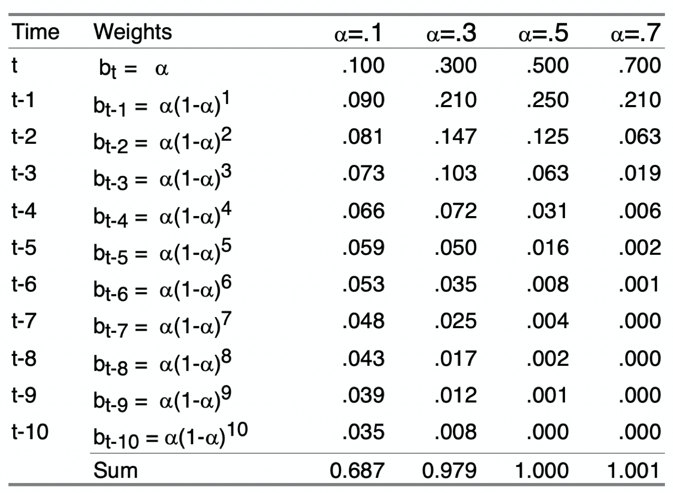
In each of the above expressions for the forecast $\hat Y_{t+1}$, the forecast is a weighted sum of some past time periods plus the forecast for the last time period considered. This pattern generalizes to all existing previous time periods. The following table in Figure 1 shows the specific values of the weights over the current and 10 previous time periods for four different values of $\alpha$. More than 10 previous time periods are necessary for the weights for lower values of $\alpha$, $\alpha = .1$ and $\alpha = .3$, to sum to 1.00.

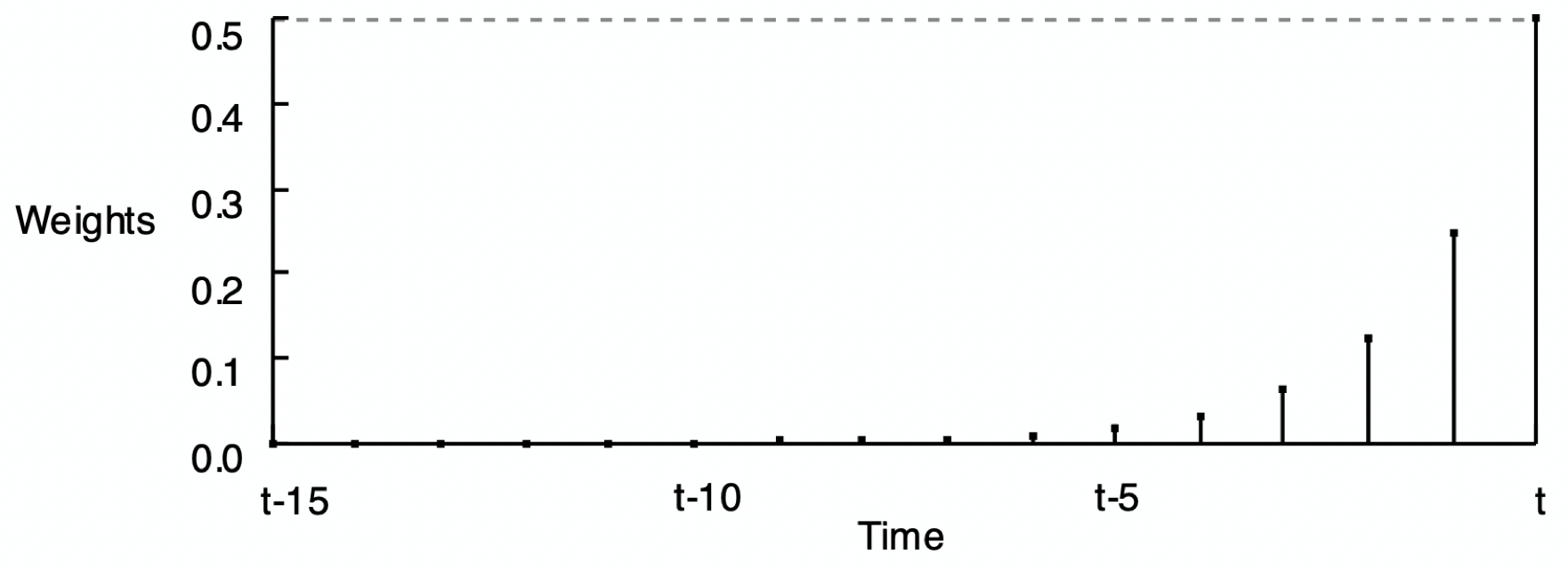
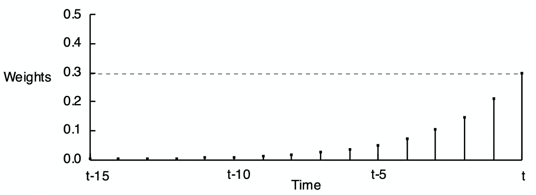
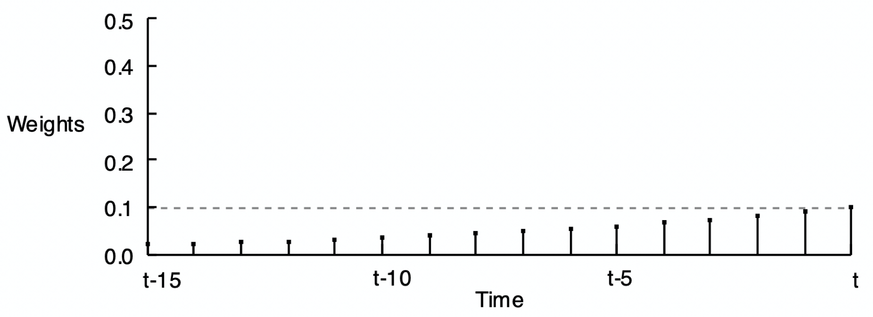
Figure 1: The weights from exponential smoothing models for alpha = .1, .3, .5, .7 for the present value of Y and the previous ten values of Y.

The reason for the word exponential in the name of this smoothing method is shown by Figure 2, Figure 3, and Figure 4 of the smoothing weights for three different values of $\alpha$. Each set of weights in the following three figures exponentially decreases from the current time period back into previous time periods.

Figure 2: Smoothing weights with alpha = .5 for the forecast of the next time period.

Figure 3: Smoothing weights with alpha = .3 for the forecast of the next time period.

Figure 4: Smoothing weights with alpha = .1 for the forecast of the next time period.

As stated, the forecast of the value of Y at the next time period is computed according to only the value of the current time period: ($\alpha$) $\hat Y_{t}$ + (1 – $\alpha$) $\hat Y_{t}$. These weights across the previous time periods are not actually computed to make the forecast, but they are implicit in the forecast and would provide the same result if the forecast was computed from all of these previous time periods.

Simple Exponential Smoothing

Refer to the exponential smoothing model described in the previous sections as simple exponential smoothing or SES. Applying the smoothing to the data results in a self-correcting model that adjusts as forecasts are made from the starting time point through the latest time period of the series. Figure 5 shows the corresponding forecast applied to a stable process.

R time series object

A time series is plotted from two variables, the dates as an R Date variable, generically labeled X, and the value of the time series at each date, generically labeled Y. We have visualized a time series by plotting the X and Y variables from within a data frame.

The R founders decided to provide another data format for representating time series data. They define this format as a time series object with type ts, created with the R function of the same name, ts(). Many functions that analyze time series data, including those we use here, analyze data as a ts object instead of two variables in a data frame.

Construct a time series object from only a single variable, a column of continuous Y values, the numerical values of the time series. The time series object specifies the date for each value of the time series without referring to any dates in the data frame even if they exist. The time series format does have the advantage of not needing access to dates in the data file, which do not need to be present.

First, read some stable process data into the d data frame.

d <- Read("http://web.pdx.edu/\~gerbing/data/Stable.xlsx")

There are four variables in this data table, each collected over time. We will focus on Variable Y3. There are no dates in the data table.

head(d)

       Y1      Y2      Y3      Y4
1 49.9994 50.0216 49.3042 47.5382
2 50.0002 50.1041 49.3760 48.8368
3 50.0006 50.0305 51.3605 51.6921
4 49.9990 49.9672 50.5292 49.7508
5 50.0022 49.9797 49.8766 50.1722
6 50.0013 50.1061 49.7658 49.6059

Using ts() to create a time series object centers on the time unit by which data were recorded. In this example, the data were recorded as quarterly data, so the time unit is one year with four periods within each year. The time unit is the length of time over which the time series data are organized that contains all of the periods (potentially seasons) without repeating a period.

In this example, convert the data in the d data frame for the variable Y3 to a ts object, with the chosen name Y_ts. Refer to the variable as d$Y3.
frequency: Parameter that indicates the number of periods in the time unit. In this example, four quarters constitute the time unit of a year, so set to the value of 4.
start: Parameter that indicates the first date of the time series, which necessarily consists of two values: The number of the first time unit, here the year, followed by the number of the period within that time unit, here the quarter. The first value in this time series was collected in Year 2017, Quarter Number 1. If the value of a parameter consists of multiple values, as it does for the start parameter, then define the multiple values as a vector grouped by the R function that defines a vector: c().

Y_ts <- ts(d$Y3, frequency=4, start=c(2017,1))

The time series object, Y_ts, is not in a data frame, so there is no d$ in front of the name of the time series object, just the name Y_ts. It is data in the form of this time series object, Y_ts, from which the exponential smoothing model is estimated as the basis for forecasting the value of future time periods.

R displays a times series object in tabular form with the data for each time unit, here a year, in each row. The columns are the periods (seasons) within each time unit, here four quarters.

Y_ts

        Qtr1    Qtr2    Qtr3    Qtr4
2017 49.3042 49.3760 51.3605 50.5292
2018 49.8766 49.7658 50.5480 50.4216
2019 49.3139 50.5413 49.1228 50.7005
2020 50.4348 49.4026 49.2185 50.2647
2021 50.3357 50.3679 50.2961 50.2833
2022 49.4608 50.7655 51.4348 51.5651
2023 49.3184 49.9858 51.1899 50.6022
2024 50.1502 49.7412

The example above is for four quarters within a year. If the data are monthly, then specify a frequency of 12, etc.

The data are available on the web at:

http://web.pdx.edu/~gerbing/data/Stable.xlsx

R simple exponential smoothing of a stable process

To do exponential smoothing, we use the ets() function from the forecast package. As with all contributed packages, the package must first be installed, such as with the RStudio Tools menu, Install Packages.... Then, in any active R session in which you refer to this function, you need to first call library(forecast).

To estimate the model, specify the time series object as the only required parameter for the ets() function. Save the results in the object with the chosen name of fit.

Model estimation: fit <- ets(Y_ts)

From the estimated model, compute the forecast with the forecast() function, also from the forecast package. Save the results in the object f. The parameter h specifies the number of time periods to forecast.

Compute the forecast: f <- forecast(fit, h=4)

Plot the time series and computed forecasts and prediction intervals from the information in the same object, here named f. As options, specify an optional title with the parameter main. Specify the label on the y-axis with the ylab parameter. You could delete both parameters if you wish.

Visualize results: autoplot(f, main=NULL, ylab="Y")

List the forecasted values and the prediction intervals as a table.

List results: f

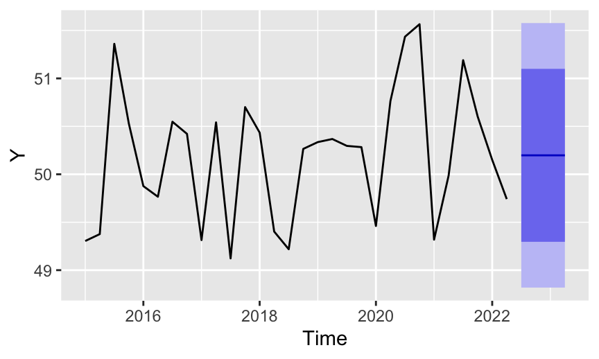
Figure 5: Simple exponential smoothing forecast applied to a stable process.

Figure 5 also visualizes the 80% and 95% prediction intervals. The wider 95% prediction interval shows in a light purple and the narrower 80% prediction interval shows in a darker shade of purple.

95% Prediction interval

Estimated range of values that contains 95% of all future values of forecasted variable Y for a given future value of time.

The 95% prediction interval is wider than than 80% prediction interval because it encompasses a larger range of potential future data values. To be more confident that the prediction interval will contain the value of Y when it occurs requires a larger prediction interval than if we are less confident. At the extreme, for data that are in the range of this example, we would be 99.9999999% confident the data value will fall within the range of -10,000 to 10,000.

In addition to the visualization, the precise forecasted values are also available along with their corresponding 80% and 95% prediction intervals.

        Point Forecast    Lo 80    Hi 80    Lo 95    Hi 95
2024 Q3       50.19771 49.29586 51.09956 48.81845 51.57697
2024 Q4       50.19771 49.29586 51.09956 48.81845 51.57697
2025 Q1       50.19771 49.29586 51.09956 48.81845 51.57697
2025 Q2       50.19771 49.29586 51.09956 48.81845 51.57697

We see that the forecasted values from the SES model are equal to each other.

\[\hat Y_{t+1} =\hat Y_{t+2} =\hat Y_{t+3} =\hat Y_{t+4} = 50.1977\] The problem is that the simple exponential smoothing model only accounts for the level of the forecasting data, the forecast from the last time point for which the value of Y exists.

Training Data

What value of $\alpha$ should be chosen for a particular model in a particular setting? Base the choice of $\alpha$ on some combination of empirical partly theoretical considerations.

The theoretical reason for the choice of the value of $\alpha$ follows from the previous table and graphs that illustrate the smoothing weights for different values of $\alpha$.

Influence of the value of $\alpha$

The larger the value of $\alpha$, the more relative emphasis placed on the current and immediate time periods.

If the time series is relatively free from random error, then a larger value of $\alpha$ permits the series to more quickly adjust to any underlying changes. For time series that contains a substantial random error component, however, smaller values of $\alpha$ should be used so as not to “overreact” to the random sampling fluctuations inherent in the data.

How to compare the utility of one value of $\alpha$ another? The answer is based on the same technique for evaluating models in general: How close is the predicted or forecasted value of Y to the actual value of Y? To fully understand the extent of this forecasting error, we need to evaluate the model against these true forecasts. How can the accuracy of a given model be evaluated when the future forecasted events have not yet occurred? There is a bit of a trick we can use before we have access to these future values of the time series. Apply the model to the data we already have, the data on which the model has been trained, that is, estimated.

Training data

Existing data values from which the forecasting model has been estimated.

For each time period of the existing time series, that is, for data that have already occurred, we can compute the value consistent with the model, the value fit by the model given previous data values that have already occurred.

Fitted values

A fitted value is the value computed by the model that estimates the next value in the time series.

When applied to future events, the value fitted by (computed from) the model is a forecast. However, when the model is applied to data that have already occurred, there is no forecast because we already know the value of Y. With imprecise language, some people refer to these fitted values that have already occurred as forecasted values. Better to be more precise. Retain the word forecast for computing the fitted value of Y from the model to future values of Y.

One issue encountered when computing the fitted values for an exponential smoothing model from the training data is that the current forecast is needed to compute the next forecast. What value should be used for the forecast of the first time period in which no previous forecast exists? One technique is to set the first forecast equal to the first data value. Another technique is to set the first forecast equal to the average of the first four or five data values.

Figure 6 shows both the data and the fitted values for both the training data and the forecasted data values. The time series of the fitted values shows the smoothing effect of the exponential smoothing model applied to the training data. Essentially, the model is used to act as if forecasting the next did the value in the time series from the previous value, even though both values have already occurred

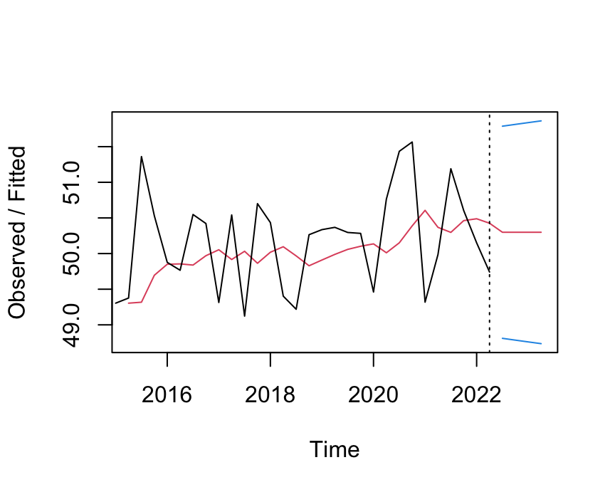
Figure 6: Simple exponential smoothing forecast applied to a stable process that illustrates data (black line) and the fitted values computed from the model (red line), which becomes the forecasted values at the end of the time series.

Assess Model Fit

For each data point, the difference between the actual data value and the value fitted by the model is the training error at that data value. The training error is computed the same as the forecasting error but applies specifically to data values on which the model trained, the training data.

For example, the third data value is for the third quarter of 2015, $Y_3=$ 51.3605, visually represented by that first peak that appears in Figure 6. The corresponding smoothed value fitted by the model, $\hat Y_3=$ 49.6959, is considerably below the corresponding data value. The model underestimates what occurred by 1.6646 units.

How do we develop a statistic that assesses the overall fit of the model to the training data? Each training data value correspondence to a fitted value, which together determine a training error. To assess the overall fit of the model to the training data, calculate this training error for each data value. The errors sum to 0 for the optimal model, so to assess the overall extent of the error, square each error and sum the squared errors. Refer to this sum as SSE, for the sum of squared errors. Because the sum depends upon the number of data values that are in the sum, We could get a smaller SSE for a bad model computed from a small amount of data than for a good model that fits the data well but is estimated from many data. So, typically convert the sum to a mean, called MSE or mean squared error.

Because the errors were squared, to obtain a fit statistic consistent with the units in which the data values are expressed, take the square root of the mean: $\sqrt{MSE}$. The result is what we call the root mean squared error or RMSE. The RMSE is a commonly used fit statistic assesses the overall fit of the model to, in this situation, the training data. No we have a guide for how we can choose the value of alpha, $\alpha$, when estimating the exponential smoothing model.

Choose the value of $\alpha$

Choose the value of $\alpha$ that minimizes RMSE $= \sqrt{MSE}$.

The discovery of the value of $\alpha$ that provides this minimization is generally provided by the exponential smoothing software. Forecasting software typically allows us to customize the value of alpha, but the value computed by the software is often the value to use. The value of $\alpha$ computed for the model visualized in Figure 6 is 0.18521, which resulted in a RMSE of 0.68. This value of $\alpha$ results in the smallest value of RMSE possible for that Version of the exponential smoothie model for that data. For example, setting $\alpha$ at 0.2 results in a RMSE of 0.726. Increasing $\alpha$ to 0.5 further increases RMSE to 0.802.

Overfitting

Unfortunately, assessing the fit of a model on the data on which it trained is a kind of cheating.

Overfitting

The model fits the training data too well, including modeling random fluctuations that do not generalize to new data for which the forecasts are made.

We do not necessarily seek the very best fit of the model to the training data. An overfit model captures too much random noise in the data. The most valid way of assessing fit is on new data. In this situation, the more interesting question is not how well the model fits the training data but rather how well it fits forecasted data. If the model is overfit, the forecasting errors will tend to be larger than the errors from the training data.

For example, are the fluctuations in the time series data regular, indicating seasonality, or are they irregular, indicating random sampling fluctuations? Particularly for smaller data sets, not only can people see patterns where none exist, so can the estimation algorithm. It is possible, for example, to submit data from a stable process and have the estimation algorithm indicate the presence of some seasonality. If this seasonality is extended into the future as a forecast, the forecasting errors will be larger if there is no seasonality in the underlying structure. An advantage in fitting the training data is not necessarily an advantage for reducing forecasting error.

More General Models

Problem with SES

The simple exponential smoothing model, or SES, with its smoothing parameter, $\alpha$, only applies to stable processes, that is, models without trend or seasonality.

Simple exponential smoothing forecast

Regardless of the form of the time series data, simple exponential smoothing provides a “flat” forecast function, all forecasts take the same value derived the last fitted value of the time series at Time t.

This flatness is fine for data without trend or seasonality, as illustrated in Figure 5 for a stable process. The problem arises when the data do possess trend and/or seasonality. Unfortunately, the simple exponential smoothing forecasts are “blind” to the trend and seasonality in the data.

Figure 7 illustrates the unresponsive flatness of the forecast of a simple exponential smoothing model, here applied to the time series data of positive trend and quarterly seasonality. The data are available on the web at:

http://web.pdx.edu/~gerbing/0Forecast/data/Sales07.xlsx

Figure 7: Inappropriate forecasts from additive trend and seasonality data with simple exponential smoothing.

The RMSE of the model is 0.394.

Forms of Exponential Smoothing

To adapt to structures other than that of a stable process, there are three primary components for defining exponential smoothing models: error, trend, and seasonality. There are two primary types of expressions for each of the three components: additive and multiplicative. The general characteristics of the resulting six different types of models are described in Table 1.

Table 1: Classification of different additive and multiplicative exponential smoothing models.

	Additive	Multiplicative
Error	The average difference between the observed value and the predicted value is constant across different levels of the time series. The error does not depend on the magnitude of the forecasted value.	The average difference between the observed and predicted values is proportional to the level of the forecasted value. As the forecasted value increases or decreases, the error also increases or decreases proportionally.
Trend	The linear trend is upwards or downwards, growing or decreasing at a constant rate, which plots as a line.	The trend component increases or decreases at a proportional rate over time. The result is an upward sloping or downward sloping curve at an accelerating rate.
Seasonal	The intensity of each seasonal effect remains the same throughout the time series, adding or subtracting the same amount from the trend component along the time series.	The intensity of each seasonal effect consistently magnifies or diminishes, adding or subtracting a increasingly larger or smaller amount from the trend component along the time series.

To generalize the simple exponential smoothing model to accommodate trend and seasonality requires the model to be expanded to include a trend parameter, respectively. Here, we will not pursue the formal statement of these more sophisticated smoothing models. Stil, the concept of a smoothing parameter remains the same, now applying not to the training error directly but to deviations from slope and seasonality estimated from the data.

The most straightforward and perhaps the most common exponential smoothing models are entirely additive. Next most common is to include a multiplicative seasonality. The accompanying reading/video illustrates these models.

What type of model is exhibited by your data? The first step is to plot your data to visually search for an underlying structure. The problem is that this structure is obscured by the random noise that contributes to each data value. With your data visualized, that is, your time series plotted, try to see through the noise and intuit the underlying structure. The better you can discern the underlying structure, the more you can guide the analytical forecasting technique too more appropriately match the existing structure. Some forecasting software will attempt to discover the additive or multiplicative structures. To better adapt to the underlying data, virtually all exponential forecasting software allows custom values of all three smoothing parameters.

Trend

To account for these deficiencies, the simple exponential smoothing models have been further refined.

Holt’s adaption of exponential smoothing to trend

Add a trend smoothing parameter to the model to account for trend in the data and the subsequent forecast.

This method provides for two smoothing equations, one for the level of the time series and one for the trend. As with the simple exponential smoothing model, the level equation forecasts as a weighted average of the current value, with weight $\alpha$ and the current forecasted value with weight $1-\alpha$. Now, however, the forecasted value is the level plus the trend.

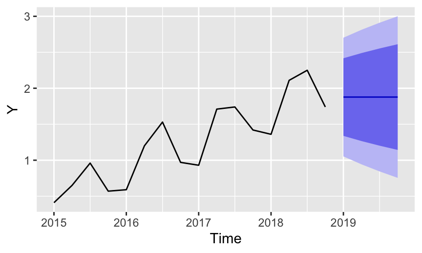
Similarly, the trend gets its own smoothing parameter, $\beta$ (beta), which follows the same logic as the $\alpha$ smoothing parameter. The trend, $\beta$, is a weighted average of the estimated trend at Time t based the previous estimate of the trend. The result is that the forecast now accounts for trend, as shown in Figure 8 of the trend and seasonal data.

R exponential smoothing with trend

The ets() function from the forecast package has an optional parameter named model. If you do not specify a value for the parameter, the function will do its best to classify your exponential smoothing model according to the three basic components: error, trend, and seasonality. The function usually gets the classification correct, but not always.

You can explicitly specify the model by specifying those three components in that order with the following codes:

"N" for no effect (except for the first component, the arrow component)
"A" for an additive effect
"M" for a multiplicative effect
"Z" for let the model decide.

For example, to specify a stable process model as in the previous example, specify a model with Additive errors, with No trend and No seasonality: "ANN". Not specifying a value for the model parameter is the same as specifying "ZZZ", that is, have the model estimate the type of error component, trend component, and seasonal component.

Specify an Additive model with Additive trend and No seasonality with "AAN".

Here, the time series object, sales_ts, has already been established.

Estimate the model: fit <- ets(sales_ts, model="AAN")

Use the accuracy() function to display several fit indices, including the root mean squared error, RMSE.

View fit indices [optional]: accuracy(fit)
Compute the forecast: f <- forecast(fit, h=4)
Visualize the forecast: autoplot(f, main=NULL, ylab="Y")
List the forecast: f

Figure 8: Inappropriate forecasts from additive trend and seasonality data accounting for trend only.

The precise fitted values and their corresponding prediction interval follow.

        Point Forecast    Lo 80    Hi 80    Lo 95    Hi 95
2024 Q1       2.127114 1.717271 2.536956 1.500314 2.753913
2024 Q2       2.229282 1.819440 2.639124 1.602482 2.856082
2024 Q3       2.331450 1.921608 2.741293 1.704651 2.958250
2024 Q4       2.433619 2.023776 2.843461 1.806819 3.060419

The corresponding fit indices follow, including the root mean squared error, RMSE. The statistic ME is the mean or average error, which should be close to zero. The statistic MAE is the mean absolute error, computed by taking the absolute value of each error term for each row of data instead of squaring the error term before summing and computing the mean. Taking the absolute value of a number just means dropping the negative sign if it exists.

             ME  RMSE  MAE    MPE   MAPE  MASE   ACF1
Training set  0 0.277 0.26 -6.008 23.356 0.641 -0.073

The model improperly ignores the seasonality but does capture the underlying trend of the data. As such the forecasted values for the next four quarters increase from 2.127 units to 2.434 units.

Trend and Seasonality

Good to account for trend, and an appropriate method for data without seasonality. Fortunately, the exponential smoothing method has also been extended to account for seasonality.

The Holt-Winters adaption of exponential smoothing to trend and seasonality

Add a trend smoothing parameter and a seasonality smoothing parameter to the model to account for trend and seasonality in the data and the subsequent forecast.

This adaption to exponential smoothing is referred to as the Holt-Winters seasonal method. This method is based on three smoothing parameters and corresponding equations — one for the level, $\alpha$ (alpha), one for the trend, $\beta$ (beta), and one for the seasonality, $\gamma$ (gamma).

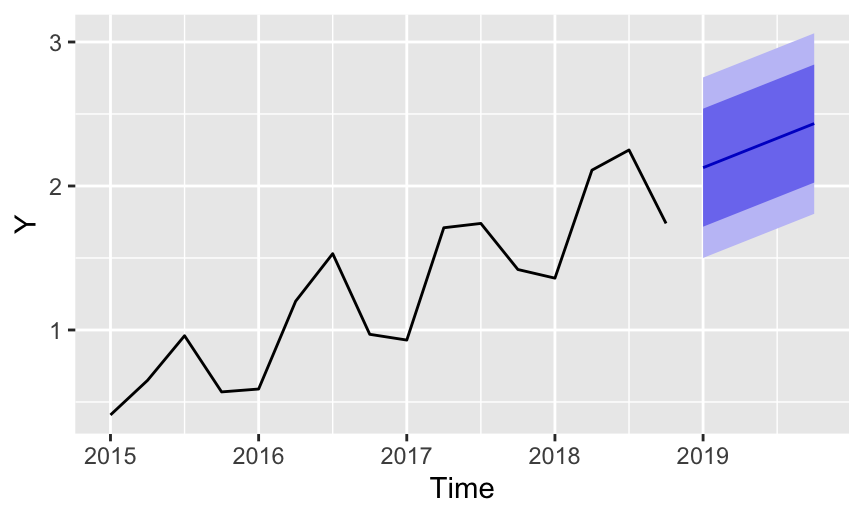
Apply the model to trend and seasonal data in Figure 9.

R exponential smoothing with trend and seasonality

You can explicitly specify the model by specifying those three components in that order with the following codes:

"N" for no effect (except for the first component, the arrow component)
"A" for an additive effect
"M" for a multiplicative effect
"Z" for let the model decide.

Specify an Additive model with Additive trend and Additive seasonality with "AAA".

Here, the time series object, sales_ts, has already been established.

Estimate the model: fit <- ets(sales_ts, model="AAA")

Use the accuracy() function to display several fit indices, including the root mean squared error, RMSE.

View fit indices [optional]: accuracy(fit)
Compute the forecast: f <- forecast(fit, h=4)
Visualize the forecast: autoplot(f, main=NULL, ylab="Y")
List the forecast: f

Get the numeric forecasts with their corresponding prediction intervals. These values can be presented as a table or as a visualization.

Figure 9: Forecasts from additive trend and seasonality with Holt-Winter’s method.

The precise fitted values and their corresponding prediction interval follow.

        Point Forecast    Lo 80    Hi 80    Lo 95    Hi 95
2024 Q1       1.838430 1.672782 2.004077 1.585094 2.091765
2024 Q2       2.433658 2.267122 2.600193 2.178963 2.688352
2024 Q3       2.635763 2.468341 2.803185 2.379713 2.891812
2024 Q4       2.190000 2.021694 2.358305 1.932598 2.447401

The corresponding fit indices follow, including RMSE.

                 ME  RMSE   MAE   MPE MAPE  MASE   ACF1
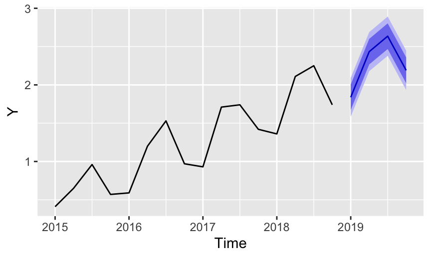
Training set -0.003 0.091 0.073 0.211 8.41 0.179 -0.436

With this more sophisticated model, although we have trend we also have seasonality where the fourth quarter tends to be lower in value than the previous quarters. Here, although there is increasing trend, Quarter #4 forecasted units are less than those forecasted for Quarter #3. Specifically, $Y_{t+3}=$ 2.636 and $Y_{t+4}=$ 2.190.

This more general model accounts for the trend and the seasonality. Because the time series is so well structured, that is, a regular pattern with relatively small random error, the forecasts show relatively small prediction intervals.

This Holt-Winters exponential smoothing forecast of this trend and seasonal data contrasts favorably with the linear regression forecast of the same data. The advantage of the Holt-Winters technique is that it does not rely upon the assumption of linearity, and so is more general. As such, it is one of the most widely used forecasting techniques in business forecasting.

We can compare the fit of the different models, each to the same data with trend and seasonality, as in Table 2.

Table 2: RMSE across three models of the same trend/seasonal data.

	Stable	Trend	Trend/Seasonality
RMSE	0.394	0.277	0.091

The more the form of the model matches the structure of the data, the better the fit to the training data. Although we do not have an estimate of true forecasting error, the same logic applies. The more data structure and model specification align, the more accurate the forecast on new data.

Appendix

The exponential smoothing model for the forecast of the next time period, t+1 is defined only in terms of the current time period t:

\[\hat Y_{t+1} = (\alpha) Y_t + (1-\alpha) \hat Y_t\]

Now, project the model back one time period to obtain the expression for the current forecast $\hat Y_t$,

\[\hat Y_t = (\alpha) Y_{t-1} + (1-\alpha) \hat Y_{t-1}\]

Now, substitute this expression for $\hat Y_t$ back into the model for the next forecast,

\[\hat Y_{t+1} = (\alpha) Y_t + (1-\alpha) \, \left[(\alpha) Y_{t-1} + (1-\alpha) \hat Y_{t-1}\right]\]

A little algebra reveals that the next forecast can be expressed in terms of the current and previous time period as,

\[\hat Y_{t+1}= (\alpha) Y_t + \alpha (1-\alpha) Y_{t-1} + (1-\alpha)^2 \, \hat Y_{t-1}\]

Moreover, this process can be repeated for each previous time period. Moving back two time periods from t+1, express the model is expressed as,

\[\hat Y_{t-1} = (\alpha) Y_{t-2} + (1-\alpha) \hat Y_{t-2}\]

Substituting in the value of $\hat Y_{t-1}$ into the previous expression for $\hat Y_{t+1}$ yields,

\[\hat Y_{t+1} = (\alpha) Y_t + \alpha (1-\alpha) Y_{t-1} + (1-\alpha)^2 \, \left[(\alpha) Y_{t-2} + (1-\alpha) \hat Y_{t-2}\right]\]

Working through the algebra results in an expression for the next forecast in terms of the current time period and the two immediately past time periods,

\[\hat Y_{t+1} = (\alpha) Y_t + \alpha (1-\alpha) Y_{t-1} + \alpha (1-\alpha)^2 \, Y_{t-2} + (1-\alpha)^3 \, \hat Y_{t-3}\]