set.seed(123)
out <- cv.glmnet(X, y, alpha=1, nfolds=10, standardize=TRUE)3 Lasso Regression
3.1 Step 2: Search for the Optimal Value of \(\lambda\)
Before running the regression regularization model, the optimal value of the lambda parameter, \(\lambda\), must be determined. The key element here is the relation between \(\lambda\) and the value of the estimated slope coefficients.
3.1.1 Cross-Validation across a Range of \(\lambda\)s
To evaluate the extent of fit for different values of \(\lambda\), function cv.glmnet() does \(k\)-fold cross-validation over select values of \(lambda\). Presumably, for each trial value of \(\lambda\), MSE on the test data is calculated for each fold, and then some average MSE value selected for that \(\lambda\) across the folds. [See Section 12.5.3 for a discussion of \(k\)-fold cross-validation.]
alpha: Set to 1 to specify Lasso regression (0 for Ridge regression and between 0 and 1 for elastic net regression).nfolds: Number of folds, with a default of 10.lambda: The default value of \(\lambda\) is for the function to select its own, but can also explicitly specify trial values of \(\lambda\) to evaluate.
The value of the alpha parameter can vary from 0 to 1. There is a more general optimization equation involving alpha that reduces to either the Ridge or Lasso criterion for respective values of 0 or 1.
Setting the seed with the R function set.seed() allows for reproducible results of selecting the \(k\)-fold samples. Generally, any pseudo-random set of values generated from any seed would be satisfactory but good to be able to reproduce the same result for comparison against different parameter values.
To view the names of all the components of the output structure, here named out, enter names(out). To view the names and their meaning, go to the section labeled Value in the manual, obtained from ?cv.glmnet.
3.1.2 Plot MSE Fit for the Trial \(\lambda\)s
Use the specialized glmnet function plot.glmnet() to plot the \(\lambda\) cross-validation results against the Mean-Squared Error (MSE). [See Section 2.5 and particularly 12.5.3 for a discussion of MSE, the variance of \(e\), \(s^2_e\), before taking the square root to get the standard deviation of residuals, \(s_e\).]
This plot function is specifically customized to produce a plot showing MSE for different values of \(\lambda\), plotted as its logarithm to produce a more compact plot. Because the class of the output data structure, out, is cv.glmnet, R recognizes that the plot should be done with the specialized function just by entering plot().
The cross-validation curve plots as a red dotted line plus the upper and lower standard deviation curves, the error bars. Each error bar represents one standard error on either side of the plotted value. [See Section 11.4.2 for a discussion of the standard error, \(s_e\).]
The plot also contains two vertical dotted lines. The first dotted line indicates the value of \(\lambda\) that yields the minimum MSE, lambda.min. The second dotted line indicates the model with the most shrinkage of the coefficients such that the test MSE is within one standard error of the minimum, lambda.1se. This second line indicates a more parsimonious model without too much of an increase of test MSE over the model with the minimum MSE, and so provides the most useful value of \(\lambda\) in most situations.
The visualization also includes the number of predictor variables retained in the model listed along the top as log(\(\lambda\)) increases.
class(out)[1] "cv.glmnet"plot(out)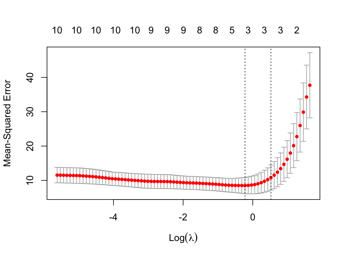
We can get the exact values of \(\lambda_{min}\) and \(\lambda_{1se}\) with print() applied to the output from cv.glmnet().
print(out)
Call:  cv.glmnet(x = X, y = y, nfolds = 10, alpha = 1, standardize = TRUE)

Measure: Mean-Squared Error

    Lambda Index Measure    SE Nonzero
min 0.8007    21    8.50 2.353       3
1se 1.6854    13   10.82 3.656       3
log(1)=0, so a negative logarithm values indicate \(\lambda < 1\).
MSE improves slightly as predictor variables are deleted from the model, from over 10 to a minimum of 8.5 for a three-predictor model. Then further deletion tends to raise MSE, dramatically after \(\lambda=1.69\). Apparently the final model will have three, or possibly two, predictor variables.
3.1.3 View Range of Trial \(\lambda\)s
This step is optional. View the actual values of \(\lambda\) that cv.glmnet() analyzed, which are stored as the lambda component of the output data structure, here out. The optional function .fmt() is from lessR internals to prevent the annoying characteristic of the R round() function of dropping trailing zeros like Excel does. The function outputs a character string that is turned back into numbers with as.numeric(). (Since we are not using lessR here, just drop the function in your own analyses.)
lambdas <- out$lambda
as.numeric(.fmt(lambdas, 3))
[1] 5.147 4.690 4.273 3.894 3.548 3.232 2.945 2.684 2.445 2.228 2.030 1.850
[13] 1.685 1.536 1.399 1.275 1.162 1.058 0.964 0.879 0.801 0.730 0.665 0.606
[25] 0.552 0.503 0.458 0.417 0.380 0.347 0.316 0.288 0.262 0.239 0.218 0.198
[37] 0.181 0.165 0.150 0.137 0.125 0.113 0.103 0.094 0.086 0.078 0.071 0.065
[49] 0.059 0.054 0.049 0.045 0.041 0.037 0.034 0.031 0.028 0.026 0.023 0.021
[61] 0.019 0.018 0.016 0.015 0.013 0.012 0.011 0.010 0.009 0.008 0.008 0.007
[73] 0.006 0.006 0.005 0.005 0.004 0.004 0.004The trial values of \(\lambda\) range from over 5 to almost 0.
3.1.4 Plot the Slopes Across the Range of \(\lambda\)s
Another optional but useful step visualizes how the slope coefficients converge to 0 as the value of \(\lambda\) increases. The plotting function is plot.glmnet(). The lessR color generation function getColors() provides the qualitative sequence of colors, each a different hue, to help distinguish the plotted curve for each predictor from the others (better than the default R color sequence). The parameter lwd specifies the width of the lines, here increased over the default value of 1 to enhance readability.
First, get the column number of each X variable to help interpret the visualization.
for (i in 1:ncol(X)) cat(i, colnames(X)[i], "\n")1 cyl
2 disp
3 hp
4 drat
5 wt
6 qsec
7 vs
8 am
9 gear
10 carb fit <- glmnet(X, y, alpha=1, lambda=lambdas, standardize=TRUE)
colors <- getColors("distinct", n=ncol(X))
plot(fit, xvar="lambda", col=colors, lwd=1.5, label=TRUE)
legend("bottomright", lwd=3, col=colors, legend=colnames(X), cex=.7)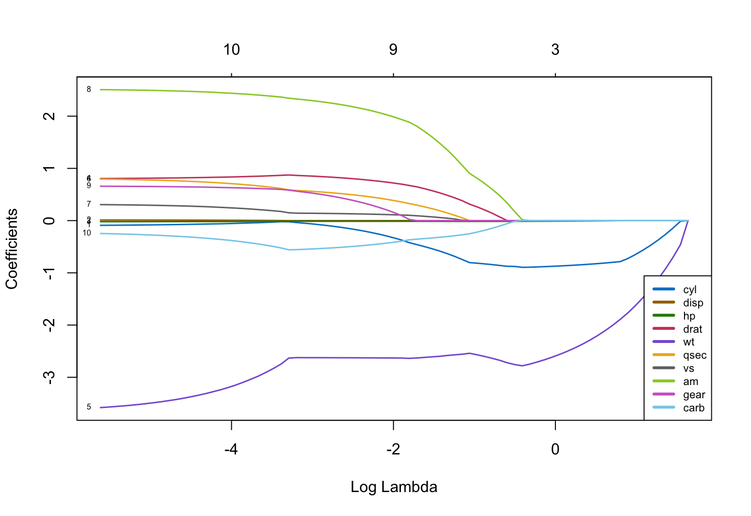
From the plot, once log(\(\lambda\)) reaches a value around 1.2, a value of \(\lambda\) around exp(1.2) = 3.32, all coefficients are 0. So \(\lambda<3\) to be useful.
The convergence of the slope coefficients to 0 is far from uniform. We can also see that the last two predictor variables remaining in the model are cyl and wt, which outlast all other coefficients through many values of \(\lambda\). From this evidence the final model may well contain just these two predictor variables.
3.1.5 Retrieve the Optimal \(\lambda\) for These Data
The value of \(\lambda\) that minimized MSE and the value that resulted in a not-much-larger MSE but provides a more parsimonious model, are included in the output structure out. The values are named lambda.min and lambda.1se, respectively. Either value of \(\lambda\), or any value between these two values, could work for deriving the final Lasso model. We choose the value that best supports parsimony. Here, also show the logarithm of the value just to place it on the previous visualization. Let’s choose the \(\lambda\) that provided a more parsimonious model. [See Section 5.2.2 for a discussion of parsimony.]
lambdaBest <- out$lambda.1se
lambdaBest
[1] 1.685404log(lambdaBest)[1] 0.5220054\(\lambda_{Best}=\) 1.685.
3.2 Step 3: Do the Lasso Regression with Chosen \(\lambda\)
3.2.1 Estimate the Model
Use lambdaBest to fit the final model with glmnet(). The default value of standardize for the X variables is TRUE, but included here for clarity. If the predictor variables are already scaled in the same units, then perhaps best to not standardize.
Again, store the results of glmnet() in a list object, here named model. Retrieve the estimated model coefficients with coef().
model <- glmnet(X, y, alpha=1, lambda=lambdaBest, standardize=TRUE)
coef(model)
11 x 1 sparse Matrix of class "dgCMatrix"
s0
(Intercept) 12.86523984
cyl -0.82245123
disp .
hp -0.00470949
drat .
wt -2.20234658
qsec .
vs .
am .
gear .
carb . The model retains cyl and wt as the predictor variables or features, and, barely, hp.
3.2.2 Evaluate Fit
Get residuals from which to compute R-squared to evaluate model fit. Function predict.glmnet() calculates the fitted values, \(\hat y\), from the model and the given values of X that remain in the model. Because the fitted model is of class glmnet, can reference the predict function simply as predict() and R will figure out what version of the function to use.
We had defined \(R^2\) as 1 minus the ratio of the SSE, the sum of squared errors, for the proposed model, to that of the flat-line null model. It turns out that this definition is equal to the correlation of the actual data values, \(y\), with the fitted data values, \(\hat y\), computed with the R function cor(), which is how \(R^2\) is computed here. [See Section 11.4.2 for a discussion of \(R^2\).]
y_hat <- predict(model, X)
rsq <- cor(y, y_hat)^2
rsq
s0
mpg 0.8382164error <- y - y_hat
m <- mean(error)
m[1] 0.000000000000001179612ersq <- error^2
SSE <- sum(ersq)
SSE[1] 286.5402MSE <- SSE / (nrow(mtcars) - 3)
MSE[1] 9.880695\(R^2=\) 0.838 for the Lasso regression model with \(\lambda=\) 1.685.
3.2.3 Explore Dropping a Variable
Horsepower, hp, just barely survived the chosen value of \(\lambda\). Its value is very close to 0 in the current solution. For comparison, raise the value of \(\lambda\) until hp effectively drops out of the model.
lambdaBigger <- lambdaBest - 0.6
model2 <- glmnet(X, y, alpha=1, lambda=lambdaBigger, standardize=TRUE)
coef(model2)
11 x 1 sparse Matrix of class "dgCMatrix"
s0
(Intercept) 14.929206261
cyl -0.865260135
disp .
hp -0.009445442
drat .
wt -2.545615327
qsec .
vs .
am .
gear .
carb . y_hat <- predict(model2, X)
rsq <- cor(y, y_hat)^2
rsq s0
mpg 0.8416704\(R^2=\) 0.842 for the Lasso regression model with \(\lambda=\) 1.085. As hp goes to 0, the coefficients for wt and cyl also shrink more and fit slightly worsens.