Lecture
8
Within Subjects/Repeated Measures/Paired t
The Concept of
Repeated Measures or Within Subjects
As you may be discovering by
now, nearly everything in statistics goes by several names. This can be
confusing and difficult, but if you understand the underlying concept, it's
easier than you might expect.
The concept of repeated measures is
pretty easy at first, but then starts to seem more complicated as you go along.
Till now, we have compared two groups on a single measure. For instance,
comparing two experimental groups on arthritis symptoms. That situation is
often called "between subjects" because some subjects in the
experiment received the new drug and some received the old drug. Comparison of
symptoms was made between different subjects. Experiments are also conducted
where the same person receives both drugs at different times. For example, a
single patient might start the study taking aspirin, then after two weeks, the
new drug is started. Symptoms in the first phase of the study are counted and
symptoms in the second phase are counted. This is called repeated measures,
because the measure is repeated for each subject.
To analyze this type of study, a
special type of statistical test is needed--the within-subjects t-test.
"Within" is used because the measure (or measures) being examined is
said to be nested within each subject. The term "within subjects" is
slightly more general than "repeated measures," because this type of
t-test is used in cases other than the repeated measures situation. For
instance, one could compare two different measures. A standardized math test
might be compared to a standardized verbal test, with the hypothesis that the
students in the sample have stronger verbal skills. Another use of the
within-subjects t-test is when subjects are linked or paired together in some
way. The best example of this is twin studies. Monozygotic twins are compared
on alcoholism or some other dimension. In this case, drinking behavior would be
analyzed as if there were repeated measurements of the same person. Each twin
pair is considered to be the same in some sense. There are several other ways
we can link pairs of subjects though, such as married couples, siblings, or
participants matched on age or some other dimension. If participants were
matched on age, all participants are first ranked according to their age, then
pairs of participants of the same (or very close) age are split into two
groups, one member or each pair assigned to each group. Each pair is then kept
linked together or "yoked."
So, there are several terms that
might be used for this type of test: within-subjects t-test, paired t-test,
matched pair t-test, or repeated measures t-test. All refer to the same type of
test in which pairs of scores are linked together and compared.
Example
Let's look at an example to see how this test is conducted. Generally, we have
the same procedures, and the same sampling variability concepts are needed.
Let's assume that a local in-home care service makes regular home visits. There
are seven nurses and nurses aids in the company that visit patients' homes to
provide assistance. The company director decides that a new visit scheduling
system should be applied that organizes visits by location to increase the
number of visits per day and thus the number of patients that can be served.
The company's service region is divided into sectors, and homes located in the
same sector are visited by one of the seven health aids on the same day. This
table presents the number of visits before and after the new system is
implemented.
|
ID# for Company's Health Aids |
Number of Visits/Day |
Number of Visits/Day |
|
1 |
3 |
6 |
|
2 |
8 |
14 |
|
3 |
4 |
8 |
|
4 |
6 |
4 |
|
5 |
9 |
16 |
|
6 |
2 |
7 |
|
7 |
12 |
19 |
We want to test whether the new
scheduling system will significantly increase the number of visits possible. To
do this, we need to test whether the increase in visits is simply a chance
occurrence or not.
Steps
Generally, we follow the same steps to conduct the significance test and find
the confidence intervals as we did with the between-groups test (also called
the "between-subjects" t-test), only the formulas are a bit
different.
|
Step Number |
Description of Step |
Specific Example with Between Groups t-test |
|
1. |
Know the hypothesis you are
testing. In this case, we are interested in the average difference between
the number of visits before and after the intervention. In the population,
that would be |
|
|
2. |
Use the formula, finding the value
of the standard error estimate first. Find the variance of difference scores
( |
|
|
3. |
Check to see if the calculated value indicates significance. To do this: determine the degrees of freedom, and look up the critical value in the table in the back of the book for alpha=.05 (in Daniel's tables, the subscript value .975 is used). If the value you calculated exceeds the value in the table, it is significant (i.e., the null hypothesis is rejected). |
d.f. = n - 1 |
|
4. |
Calculate the 95% confidence interval. Two values are used: (1) the low value, which subtracts the product of the critical value times the standard error, and (2) the high value, which adds that product. |
|
Computations
|
ID |
Before |
After |
|
|
|
|
1 |
3 |
6 |
3 |
-1.29 |
1.66 |
|
2 |
8 |
14 |
6 |
1.71 |
2.92 |
|
3 |
4 |
8 |
4 |
-.29 |
.08 |
|
4 |
6 |
4 |
-2 |
6.29 |
39.56 |
|
5 |
9 |
16 |
7 |
2.71 |
7.34 |
|
6 |
2 |
7 |
5 |
.71 |
.50 |
|
7 |
12 |
19 |
7 |
2.71 |
7.34 |
![]() ,
, ![]() ,
, ![]() 59.40
59.40
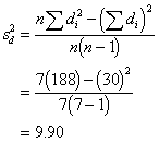
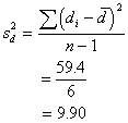
I'll calculate the variance of the
difference both ways, but you don't have to.
|
|
|
Now, the standard error of the
differences.

And the t value:

To see if this computed value is
significant, we should compare it to the tabled value (Table E), looking up
under d.f. = n - 1 = 6. The critical value to exceed is t.975 =
2.4496. Because our calculated value of t for the sample, 3.61, is larger than
2.4496 found in the table, we decide our difference is large enough and therefore
significant. We reject H0 which stated that there was no difference
between before and after measurements.
Interpretation
Note that there is a similarity between this t formula and the between-subjects
t formula. Essentially, we are finding a ratio of the average differences
between scores relative to sampling variability. So, the average difference (![]() ) is divided by
the standard error of the difference
) is divided by
the standard error of the difference ![]() .
.
The unique thing about this test is
that we compare every individual's score to his/her other score, by subtracting
the second score from the first (![]() ). Then we find the average of that. In the
between-groups t-test, we computed the mean of score for one group and then
compared it to the mean score of the other group. With the within-subject
approach differences are found first, then the average, and with the
between-subjects we find the average first, then the difference.
). Then we find the average of that. In the
between-groups t-test, we computed the mean of score for one group and then
compared it to the mean score of the other group. With the within-subject
approach differences are found first, then the average, and with the
between-subjects we find the average first, then the difference.
Advantages of the
Within-subjects t-test.
When a within-subjects test is conducted, every participant has his or her own
little control group, whether it is the same person being measured a second
time, or it is an MZ twin. This means that for each person, all factors are
held constant except whatever happened between the two measurements. With
repeated measures, it is the same person, and presumably the only thing that
differed between the first measure and the second, is whatever happened in
between (e.g., the intervention). With twins, the genetics are all the same, so
any differences in drinking behaviors between pairs are a result of
environmental influences.
Because each person (or pair) has
his or her own control, we will have less overall variation in the sample than
if we compare different people in two different groups. And because we can
reduce the overall variation, the estimate of sampling variability will be
smaller (remember that ![]() is estimated using the variability in the sample,
is estimated using the variability in the sample, ![]() ). In other
words,
). In other
words, ![]() will
generally be smaller than
will
generally be smaller than ![]() .
.
In general, within-subjects tests
designs have this advantage over the between-subjects designs. Within -subjects
designs have more power to detect significance because there is less
variability. If it is ethically or methodologically possible to do, an experiment
with a within-subjects design is more powerful and economical than a
between-subjects experiment.
For an example SPSS output click here.


