Lecture
7
Example of Between Groups t-test
As an example, let us consider a
hypothetical research study that examines dispositional characteristics of
children born first or second in a family. Twenty children are surveyed on
their level of introversion to see if children born first are more likely to be
introverted than children born second (perhaps because they don't have a
sibling to play with in the first couple of years). The scores on the
introversion test have possible values of 0 to 100, with higher scores
indicating more introversion. Here are the data for our sample of twenty:
|
Child ID |
Born first or
second |
Introversion score |
|
1 |
1 |
65 |
|
2 |
1 |
48 |
|
3 |
1 |
63 |
|
4 |
1 |
52 |
|
5 |
1 |
61 |
|
6 |
1 |
53 |
|
7 |
1 |
63 |
|
8 |
1 |
70 |
|
9 |
1 |
65 |
|
10 |
1 |
66 |
|
11 |
2 |
61 |
|
12 |
2 |
42 |
|
13 |
2 |
66 |
|
14 |
2 |
52 |
|
15 |
2 |
47 |
|
16 |
2 |
58 |
|
17 |
2 |
65 |
|
18 |
2 |
62 |
|
19 |
2 |
64 |
|
20 |
2 |
69 |
Conducting the
Significance Test
I'm going to cheat a little and assume that the variances and means for each
have already been computed: ![]() = 50.93 and
= 50.93 and ![]() = 78.27 and
= 78.27 and ![]() = 60.6 and
= 60.6 and ![]() = 58.6.
= 58.6.
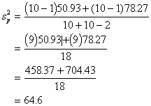
We start by figuring out the pooled
variance estimate where the variances for the two groups are put together. For
that we use this formula,
![]()
in which ![]() are the variances for the two
groups, and
are the variances for the two
groups, and ![]() are
the sample sizes for each group. Plugging these numbers in we get:
are
the sample sizes for each group. Plugging these numbers in we get:

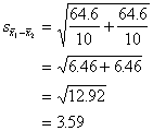
Now, to the standard error, whose
formula looks like this:

And plugging in the values we
already have,

Since we now have the standard
error and we were given the means for the two groups before, we can get the
t-value.

To see if the difference between the
means is extreme enough to be significant at a = .05, we look up in
the t-table in the back of the text (Table E) under d.f. = n1 + n2
- 2 = 10 + 10 - 2 = 18, using the column t.975 because we are doing
a two-tailed test with a = .05. The corresponding number in the body
of the table is 2.1009. Our calculated t-value, .56, does not excede this
number from the table, so it is not extreme enough. We conclude that the
difference between the two groups is nonsignificant at p < .05. In other
words, we decide to retain the null hypothesis that says that, in the
population, first and second children are equally introverted.
Confidence
Intervals
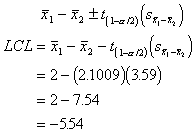
We could have also done this test by calculating the 95% confidence interval
and checking to see if we would predict that the group difference in the
population would be greater than zero. To do this, we use the previously
obtained values to compute the LCL and UCL (upper and lower confidence levels).
The formula for the confidence intervals looks like this:

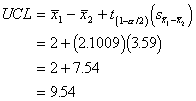
The UCL is pretty easy once we've
done this:

The confidence limits are -5.54 and
9.54, and because they contain the number 0, that means that the difference
between the two group means in the population could be 0. So, we can't be sure
that there will be a difference in the population. That leads us to the same
conclusion, that in the sample the group means are not significantly different
from one another.
To see an SPSS example printout
click here.