Lecture
5
Normal and Binomial Probability Distributions
I'm going to use this lecture to tie
together some loose ends as well as briefly discuss the theoretical
distributions that are going to be lurking in the background of everything we
do this quarter.
Normal Distribution
Hopefully, the normal
distribution is old hat to you. The normal distribution has some particular
mathematical properties which we'll leave for the mathematicians. But basically
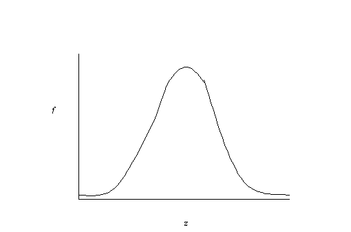
it looks something like this:

The normal distribution is a very
useful distribution. From it's shape, we can figure out the area under the
curve (for you calculus buffs, this should sound familiar). The area under the
curve is useful because when the curve is a frequency distribution, the area
can tell us the number of people in the sample that are at or below a certain
value on the x-axis (uh… remember, the horizontal one). So, if the x-axis
represents values of test scores or something we care about, the area can tell
us the number or percentage of people with test scores above or below a certain
test score. z-scores are special scores that relate to normal curves.
The standard normal curve is a frequency distribution just like the one
pictured above, with a mean value of z = 0 and a standard deviation of
1. Because z-scores, normal curves, and this calculus stuff pertaining to area
under the curve are all related, we know that a certain z-score has a certain
percentage of people in the frequency distribution above or below that z value.
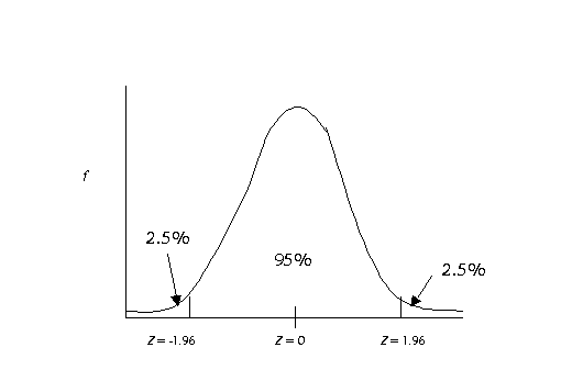
There is one z-score in particular that is important, it is a z = 1.96 (-1.96
is also important). The reason why 1.96 is so important is that 95% of the
people in a given sample or population have z-scores between -1.96 and 1.96.

The really nice thing about all of
this is that if the normal distribution we are talking about is a sampling
distribution, we know how many samples will have values between certain
z-scores. Remember that the central limit theorem as discussed in the previous lecture
states that sampling distributions will be approximately normal regardless of
the shape of the population distribution. So, by knowing the properties of the
normal curve, we can tell just how rare our sample is likely to be.
In the third lecture on significance testing,
I told you that alpha, by convention, is set equal to .05. When discussing
sampling distributions, alpha corresponds to 5% of the samples in the sampling
distribution. So, we consider some statistic significant if its probability of
occurring by chance (i.e., because of random sampling variability) is less than
5%. This is usually stated as p < .05 (where p stands for
probability). Take for instance a sample mean, if the mean of a sample is way
out on the tail of the distribution of all possible samples (i.e., the sampling
distribution), its pretty rare, and we consider it to be statistically
significant. So, if the z value is greater than 1.96 or less than -1.96, it's
significant (p < .05).
(As an aside, this is called a
two-tailed test, because we have split the 5% into the upper and lower half.
The one-tailed test puts all of the 5% into one side, so the sample mean does
not have to be as extreme to be considered significant. Many people, including
myself, are critics of the one-tailed test. We are critical primarily because
the usual standard is a two-tailed probability for significance. If someone
reports a one-tailed test of significance, it sounds like the result is
significant at p < .05 (one-tailed), but the statistic does not have to be
as extreme to be significant. p < .05, one-tailed, is actually equal to p
< .10, two tailed.)
z's Cousin, the t
Distribution
The t-distribution is very similar to the z-distribution. It is used because
the sampling distribution shape is a little flatter when we have small samples
(as described in the lecture on sample size).
So the t-distribution is really just an adjustment of the z-distribution for
sample size. Take a second right now to crack open your textbook to Table E in
the back. Look under the column t.975 because that corresponds to
the point on the curve at which only 2.5% of the samples are larger (p <
.05, two-tailed). Look at the values in this column and follow them down the
page. As the d.f. (degrees of freedom) increases, the t-values get smaller.
Degrees of freedom are based on sample size (usually n-1 or n-2).
So, as the sample size gets larger, the t decreases. As the sample size
reaches infinity (sideways 8) the value of t reaches 1.96. So, if your
sample size is above 200 (the second to the last row), the t-distribution is
equal to the standard normal z-distribution.
Binomial
Probability Distribution
Up to this point, most of my
examples have dealt with measures (or variables) that fall into our general
category of "continuous." When categorical (or dichotomous) variables
are analyzed, we rely on the binomial distribution. The binomial distribution
has to do with the probability of a yes/no type of occurrence--either something
occurs or it does not. This might pertain to the probability of responding
"yes" or the probability of a coin turning up heads when it is
flipped. Let's consider the coin toss for now. In a single toss, there is a
50/50 chance the coin will come up heads. If we toss it five times, there are a
number of possible outcomes. We might have 5 heads in a row, 4 out of the 5
tosses might be heads, 3 out of the five tosses might be heads and so on. It
seems unlikely that we would get 5 heads or 0 heads, that's pretty rare. Its
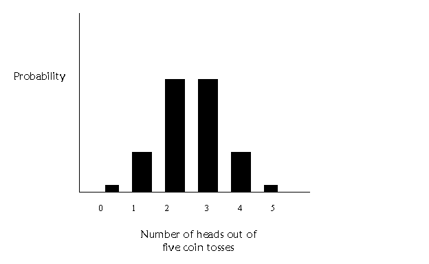
more likely we will get some of each. This table contains the probability of
each of these occurrences:
|
Number of heads out of 5 tosses |
Probability of this occurring |
|
5 |
.03 |
|
4 |
.16 |
|
3 |
.31 |
|
2 |
.31 |
|
1 |
.16 |
|
0 |
.03 |
(note: if this doesn't sound
familiar to you, look through Chapter 3). Getting 5 and 0 are equally likely
and rare. Getting 2 or 3 are equal but more likely than getting 5 or 0. If we
plot the probability by each occurrence, we get a graph that looks like this:

Ok, instead of coin tosses, we could
think of taking a random sample of size five. Assume that we have a 50/50
chance of each person in the sample being female or male. The probability that
the sample will have 5 females or 5 males will be pretty low. The probability
of having a few of each will be higher. Now assume, that we take lots and lots
of samples of size five from a population, and for each sample, we count up how
many people in each sample are male and female. Samples with all males and all
female will be rarer and samples with a few of each will be more common. Voila!
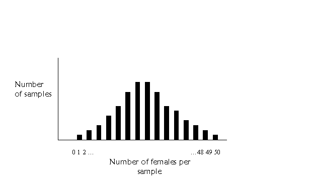
You have a binomial sampling distribution!
One more thing…if we have larger
samples, say of 50 or so, there will be many more bars on the graph. It might
look something like this:

Starting to look kind of
familiar?……….