Lecture
21
Logistic
Regression
Logistic regression is a predictive
analysis, like linear regression, but logistic regression involves prediction
of a dichotomous dependent variable. The predictors can be continuous or
dichotomous, just as in regression analysis, but ordinary least squares
regression (OLS) is not appropriate if the outcome is dichotomous. Whereas the
OLS regression uses normal probability theory, logistic regression uses
binomial probability theory. This makes things a bit more complicated
mathematically, so we will only cover this topic fairly superficially (believe
me, I'm mixing it with sugar!).
Chi-square and
Logistic Regression
Because the binomial
distribution is used, we might expect that there will be a relationship between
logistic regression and chi-square analysis. It turns out that the 2 X 2
contingency analysis with chi-square is really just a special case of logistic
regression, and this is analogous to the relationship between ANOVA and
regression. With chi-square contingency analysis, the independent variable is
dichotomous and the dependent variable is dichotomous. We can also conduct an
equivalent logistic regression analysis with a dichotomous independent variable
predicting a dichotomous dependent variable. Logistic regression is a more
general analysis, however, because the independent variable (i.e., the
predictor) is not restricted to a dichotomous variable. Nor is logistic
regression limited to a single predictor.
Let's take an example. Coronary
heart disease (CHD) is an increasing risk as one's age increases. We can think
of CHD as a dichotomous variable (although one can also imagine some continuous
measures of this). For this example, either a patient has CHD or not. If we
were to plot the relationship between age and CHD in a scatterplot, we would get
something that looks like this:
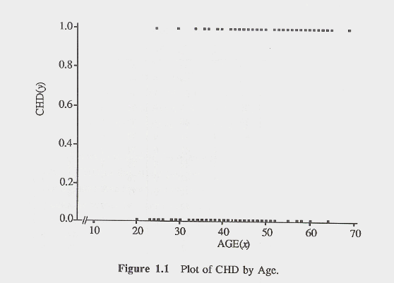
We can see from the graph that there
is somewhat of a greater likelihood that CHD will occur at older ages. But this
figure is not very suitable for examining that. If we tried to draw a straight
(best fitting) line through the points, it would not do a very good job of
explaining the data. One solution would be to convert or transform these
numbers into probabilities. We might compute the average of the y values at
each point on the x axis. The y values can only be 0 or 1, so an average of
them will be between 0 and 1 (.2, .9, .6 etc.). This average is the same as the
probability of having a value of 1 on the y variable, given a certain value of
x (notated as P(y|xi). So, we could then plot the probabilities of y
at each value of x and it would look something like this:
This is a smoother curve, and it is
easy to see that the probability of having CHD increases as values of x
increase. What we have just done is transform the scores so that the curve now
fits a cumulative probability curve for the logistic distribution. As
you can see this curve is not a straight line; it is more of an s-shaped curve.
This s-shape, however, resembles some statistical distributions that can be
used to generate a type of regression equation and its statistical tests.
The Logistic
Regression Equation
If we are to get from a straight line (as in regression) to the s-curve (as in
logistic) in the above graph, we need some further mathematical
transformations. What we get is an ugly formula with a natural logarithm in it:
![]()
This formula shows the relationship
between the regression equation (a + bx), which is a straight line formula, and the
logistic regression equation (the ugly thing on the left). The ugly formula
(some twisted folk would say it is beautiful) involves the probability, p, that
y equals 1 and the natural logarithm, a mathematical function abbreviated ln.
In the CHD example, the probability that y equals 1 is the probability of
having CHD if you are a certain age. p can be computed with the following
formula:
![]()
The above formula, called the logit
transformation, uses an abbreviation for exponent (exp), another mathematic
function. Don't worry, I will not ask you to calculate the above formulas by
hand, but if you had to, it would not be as hard as you think. My purpose is to
expose you to the formulas so you have some idea how the we get from a
regression formula for a line to the logistic analysis and back. You see,
logistic regression analysis follows a very similar procedure to OLS
regression, only we need a transformation of the regression formula and some
binomial theory to conduct our tests.
A Brief Sidebar on
exp and ln
exp, the exponential function, and ln, the natural logarithm are opposites. The
exponential function involves the constant with the value of 2.71828182845904
(roughly 2.72). When we take the exponential function of a number, we take 2.72
raised to the power of the number. So, exp(3) equals 2.72 cubed or (2.72)3
= 20.09. The natural logarithm is the opposite of the exp function. If we take
ln(20.09), we get the number 3. These are common mathematical functions on many
calculators.
Model Fit and the
Likelihood Function
Just as in regression, we can find a best fitting line of sorts. In regression,
we used a criteria called ordinary lease squares, which minimized the squared
residuals or errors in order to find the line that best predicted our swarm of
points. In logistic regression, we use a slightly different system. Instead of
minimizing the error terms with least squares, we use a calculus based function
called Maximum Likelihood (or ML). ML does the same sort of thing in logistic
regression. It finds the function that will maximize our ability to predict the
probability of y based on what we know about x. In other words, ML finds the
best values for the formulas discussed above to predict CHD with age.
The Maximum Likelihood function in
logistic regression gives us a kind of chi-square value. The chi-square value
is based on the ability to predict y values with and without x. This is similar
to what we did in regression in some ways. Remember that how well we could
predict y was based on the distance between the regression line and the mean
(the flat, horizontal line) of y. Our sum of squares regression (or explained)
is based on the difference between the predicted y and the mean of y(![]() ). Another way
of stating this is that regression analysis compares the prediction of y values
when x is used to when x is not used to predict them.
). Another way
of stating this is that regression analysis compares the prediction of y values
when x is used to when x is not used to predict them.
The ML method does a similar thing.
It calculates the fitting function without using the predictor x and then
recalculates it using what we know about x. The result is a difference in
goodness of fit. The fit should increase with the addition of the predictor
variable, x. Thus, a chi-square value is computed by comparing these two models
(one utilizing x and one not utilizing x).
The conceptual formula looks like
this, where G stands for "goodness of fit":
![]()
Mathematically speaking, it is more
precisely described as this:
![]()
and, as a result, sometimes you will
see G referred to as "-2 log likelihood" as SPSS does. G is
distributed as a chi-square statistic with 1 degree of freedom, so a chi-square
test is the test of the fit of the model. As it turns out, G is not exactly
equal to Pearson chi-square, but it usually lead to the same conclusion.
Odds Ratio and b
As we can see from the logistic equation mentioned earlier, we can obtain
"slope" values, b's, from the logistic equation. These, of course,
are a result of our transforming equations that allowed us to get from the
logistic equation to the regression equation. The slope can be interpreted as
the change in the average value of y, from one unit of change in x.
The odds ratio is also obtained from
the logistic regression. It turns out that the odds ratio is equal to the
exponential function of the slope, calculated as exp(b). The odds ratio is
interpreted as it is with the contingency table analysis. An odds ratio of 3.03
indicates that there is about a three-fold greater chance of having the disease
given one unit increase in x (e.g., 1 year increase in age). If this was the
ratio obtained from the age and CHD example, the odds ratio would indicate a
3.03 times greater chance of having CHD with every year increase in age.
It is relatively easy to convert
from the slope, b, to the odds ratio, OR with most calculators.

A Note on Coding of
Y and X
One quick note on coding. It is
important to code the dichotomous variables as 0 and 1 with logistic regression
(rather than 1 and 2 or some other coding), because the coding will affect the
odds ratios and slope estimates.
Also, if the independent variable is
dichotomous, SPSS asks what coding methods you would like for the predictor
variable (under the Categorical button), and there are several options to
choose from (e.g., difference, Helmert, deviation, simple). All of these are
different ways of dummy coding that will produce slightly different results.
For most situations, I would choose the "indicator" coding scheme.
Usually, the absence of the risk factor is coded as 0, and the presence of the
risk factor is coded 1. If so, you want to make sure that the first category
(the one of the lowest value, which is 0 here) is designated as the reference
category in the categorical dialogue box.
SPSS Printout
I computed a logistic regression
analysis with SPSS on the Clinton referendum example (Lecture 13). In that
example, our imaginary study asked people twice whether they think President
Clinton should be removed from office. The logistic regression used their
responses on Time 1 to predict their responses at Time 2. Click here for the annotated printout.