Lecture 15
Point-biserial
correlation, Phi, & Cramer's V
Differences and
Relationships
The correlation coefficient is a measure of how two variables are related. t-tests
examine how two groups are different. What if I told you these two types of
questions are really the same question?
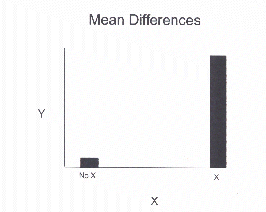
Examine the following histogram.
This histogram shows a large difference in the dependent variable, y, between
the groups No X and X. The mean is much higher for the X than the No X group.

This is an example in which X has
two groups. Now imagine that there are several values (levels or groups) for
variable X: No X, a little X, some X, a lot of X, all of X. For instance, what
if instead of having a study with no drug vs. drug, there is a study in which
several levels of dosage used (e.g., 0mg, 5mg, 10mg, etc). Then there would be
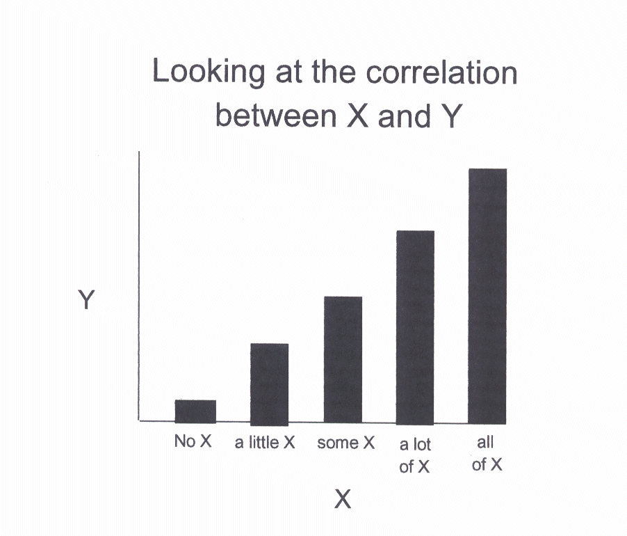
several intermittent values of X. The following graph shows one potential
outcome of the study in which there are several levels of X.

In this second graph, we see that as
the value of X increases, the value of Y increases. That is the definition of a
relationship. In other words, there is a correlation between X and Y.
The same holds true for the first
figure in which there were only two values of X. As X increases, Y increases.
So both graphs demonstrate that there is a relationship between X and Y. At the
same time, we can see that both graphs demonstrate that the values of Y differ
for the values of X. So, a difference between values of X is the same as a
relationship between X and Y.
Point-biserial
Correlation
A point-biserial correlation is simply the correlation between one
dichotmous variable and one continuous variable. It turns out that this is a
special case of the Pearson correlation. So computing the special
point-biserial correlation is equivalent to computing the Pearson correlation
when one variable is dichotmous and the other is continuous.
Because we know that differences are
the same as correlations now, we can show that the t-test for two groups is the
same as the correlation between the grouping or independent variable (X) and
the dependent variable (Y). Let's go back to our last t-test example and check
this out. In this example, we were comparing first and last siblings
to see who was more introverted.
|
First or Last Sibling |
Introversion |
|
1 |
65 |
|
1 |
48 |
|
1 |
63 |
|
1 |
52 |
|
1 |
61 |
|
1 |
53 |
|
1 |
63 |
|
1 |
70 |
|
1 |
65 |
|
1 |
66 |
|
2 |
61 |
|
2 |
42 |
|
2 |
66 |
|
2 |
52 |
|
2 |
47 |
|
2 |
58 |
|
2 |
65 |
|
2 |
62 |
|
2 |
64 |
|
2 |
69 |
When we conducted the t-test we got
the following results:

This t-value was non-significant,
indicating no significant differences between the groups.
If we compute a correlation between
the grouping variable (sibling) and the the introversion score for this same
data, the r= -.13 (I magically arrived at this figure with some assistance from
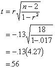
my friend Hal). If we plug this into the t-test formula used for testing the
significance of a correlation, we would get this:

which is the very same t-value from
the difference test above. The correlation test (also nonsignificant) indicates
that there is no relationship between the sibling group and the introversion
score.
So, a difference is a correlation.
Phi
There is another special case of correlation called "phi" (or f,
the Greek letter f ). Phi represents the correlation between two dichotmous
variables. As with the point-biserial, computing the Pearson correlation for
two dichotomous variables is the same as the phi.
Similar to the t-test/correlation
equivalence, the relationship between two dichotomous variables is the same as
the difference between two groups when the dependent variable is dichotmous.
The appropriate test to compare group differences with a dichotmous outcome is
the chi-square statistic. And, we can also show that the test of the phi
coefficient is equivalent to the chi-square test.
Remember, one of the ways chi-square
is interpreted is as a test of independence. The test of independence refers to
whether or not two varables are related. If two variables are related, they are
correlated.
So, when we conduct a chi-square
test, and we want to have a rough estimate of how strongly related the two
variables are, we can examine phi. Squaring phi will give you the approximate
amount of shared variance between the two variables, as does r-square.
Cramer's V
Cramer's V is used to examine the association between two categorical variables
when there is more than a 2 X 2 contingency (e.g., 2 X 3). In these more
complicated designs, phi is not appropriate, but Cramer's statistic is.
Cramer's V represents the association or correlation between two variables.
I've also seen this statistic referred to as "Cramers Phi".