Lecture 13
More on Chi-square
There are several
loose ends on chi-square that I would like to tie up.
Simple Chi-square
Problems
My discussion thus far has primarily focused on the 2 X 2 contingency table
which looks at the goodness-of-fit or the independence of two dichotomous
variables. I skipped a simpler example of chi-square which I would like to
return to now.
A very easy and simple
example of chi-square is when the frequencies of response to one dichotomous
variable are compared. For this, we have just one variable that is tested.
Examples of this are very common in the newspapers when polls are published.
For instance, we might conduct a statewide survey of a sample of 300 hospital
workers and ask the question "Do you think that staffing is adequate at
your hospital, yes or no?" The following might be a hypothetical result:
|
No |
Yes |
|
180 |
120 |
The chi-square test
asks if frequency of no responses is statistically larger (or different) from
the frequency of yes responses. To compute this, we first need to know the
expected frequency. Because we expect equal to imply a .5 chance of answering
no or yes, we should expect half, or 150, of the survey participants to say yes
or no. Thus we have this table of observed and expected frequencies:
|
|
No |
Yes |
|
Oi |
180 |
120 |
|
Ei |
150 |
150 |
We then apply our
usual chi-square formula:
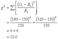
The degrees of
freedom for this test is just the number of columns - 1 (c - 1 = 1). The
critical value to exceed is equal at a
= .05 is 3.84. Thus, respondents were significantly more likely to say no than
yes to the question about adequate staffing.
This test can be
conducted another way, using proportions. Usually survey responses are reported
as the percentage (or, less often, proportion) of respondents indicating yes or
no. These same results could be described as 60% indicating no and 40%
indicating yes. The test to see whether these proportions are different is also
appropriate for this example:
![]()
where ![]() is
the obtained proportion and
is
the obtained proportion and ![]() (the Greek letter pi) is the proportion expected in the
population (usually .5), and n is the sample size for the whole sample.
Plugging in our results we get:
(the Greek letter pi) is the proportion expected in the
population (usually .5), and n is the sample size for the whole sample.
Plugging in our results we get:
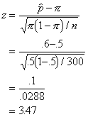
Because chi-square
and z are related, we should be able to show the equivalence of the two tests:
![]()
And, within
rounding error, this is the answer we got when we used the chi-square test of
frequencies. The nice thing about the proportion test is that we can calculate
a "margin of error" by computing our confidence intervals. I will
just compute the UCL here.
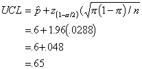
This computation
indicates that we can expect our survey to be accurate within about .048 or 5%
on either side, because the confidence limits span from .55 to .65. This is the
"margin of error" that is often reported with surveys in the media.
Of course, the same
equivalence holds for the chi-square with at 2 X 2 contingency table and the
test of two proportions that is presented in the book.
Post Hoc Follow-up
Tests
Another
chi-square topic concerns follow-up or post hoc tests when a larger contingency
table (e.g., 3 X 3) is analyzed. Just like with the ANOVA test, the chi-square
test is an "omnibus" test, because it is an overall test to see if
there are differences between any of the cell frequencies. If just two of the
cells in the design are significantly different, the omnibus test will be
significant.
It is appropriate
to conduct follow-up chi-square tests if one wants to discover which pairs of
cells are significantly different. In conducting follow-up tests, some
statisticians like to distinguish between "post hoc" follow-up tests
and "a priori" tests. "Post hoc" means after the fact, and
"a priori" means prior or planned ahead of time. The post hoc test is
one that is not planned before the initial test and usually involves many or
all possible comparisons. A priori tests on the other hand are typically fewer
in number and test specific cell differences within the design that were
predicted ahead of time.
For the post hoc
tests, authors like to recommend a correction for problems with alpha
inflation. In order to compensate for the alpha inflation problem, a researcher
can set the alpha value required for significance to a lower value. The formula
that is often used is called Bonferroni's correction and corrects for the
number of chi-square tests and the d.f. involved in each test (actually this is
a modified Bonferroni test suggested by Keppel). If we conducted 10 follow-up
tests, each with d.f. = 1, we would use:
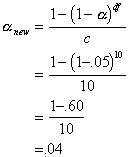
So, we need to
reset alpha to .04 to account for alpha inflation when conducting 10 single
degree of freedom tests. Notice that alpha inflation is not that large for this
many tests.
Within-subjects
Chi-Square
There is a
within-subjects version of the chi-square test. Imagine a study in which
participants repeated the same measure twice, and the measure is a dichotomous
one. In this case, the usual chi-square test is not appropriate, because we
have a within-subjects design. Let's use the previous example of the hospital
survey, but let's assume we first survey the 300 staff members before some
important reorganization of staff is implemented. Then we resurvey them to see
if their attitudes are changed. Notice that the frequency table looks similar
to the 2 X 2 contingency table we had before. However, there is an important
difference, and that is the fact that the measurements are repeated on the same
group of 300. Our sample size is still 300 total.
|
|
|
Time 2 |
|
|
|
|
|
No |
Yes |
Total |
|
Time |
No |
80 |
100 |
180 |
|
1 |
Yes |
10 |
110 |
120 |
|
Total |
|
90 |
210 |
300 |
The test for this
is simple. It is also a chi-square test, but it is called McNemar's chi-square
test. If we label our cells like before, we can use a simple computational
formula.
|
|
|
Time 2 |
|
|
|
|
No |
Yes |
|
Time |
No |
a |
b |
|
1 |
Yes |
c |
d |
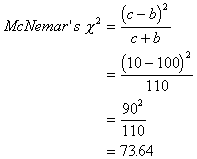
This is a d.f.=1
test, and the critical value at a
= .05 is 3.84. Thus, the change in opinions about staffing was wildly
significant (sarcasm implied with the term "wildly").
Be careful about
how you set up this table. Notice first that the cells represent a cross of
people who said no on the first occasion and yes on the second occasion etc.
Also, whether c is subtracted from b or a from d depends on how one sets up the
table. One could list Yes first and No second, for instance. What you should
keep in mind is that the test is based on the discordant cells (yes at
Time 1 and no at Time 2; or no at Time 1 and yes at Time 2). Furthermore, it
really does not matter what order the discordant cells are subtracted or added
in the formula. We could have subtracted c from b instead. Because we square
the difference, it makes no difference which is subtracted from which.
Multi-way Frequency
Tables
Like factorial ANOVA, we can also examine two independent variables with
chi-square. Our example in the 2 X 2 chi-square in the previous lecture
involved gender differences in political affiliation. One can think of this as
an independent variable of gender and a dichotomous dependent variable of
political affiliation. We could complicate this by examining the same problem,
but comparing regions (e.g., northern states to southern states). Our results
might look like this:
Northern
|
|
Females |
Males |
Total |
|
Democrats |
50 |
70 |
120 |
|
Republicans |
19 |
41 |
60 |
|
Total |
69 |
111 |
180 |
Southern
|
|
Females |
Males |
Total |
|
Democrats |
70 |
30 |
100 |
|
Republicans |
20 |
80 |
100 |
|
Total |
90 |
110 |
200 |
One can think of
the region variable as another independent variable. Does the effect of gender
on political affiliation depend on the region the voter is from? In other
words, is there an interaction between two independent variables. Notice,
however, that the 2 X 2 X 2 contingency analysis is really analogous to the 2 X
2 ANOVA, because one of the 2's is the dichotomous outcome.
There are several
ways to analyze this more complex design. One way is through a special
chi-square that tests the equivalence of the two 2 X 2 contingency tables.
Unfortunately, this test is not discussed or used very frequently, and is not
available in SPSS. A second way to analyze this data is to compare the relative
risk in the Northern region and the Southern region. That analysis compares two
odds ratios and involves testing the interaction with logistic regression. We
will briefly discuss this in a later section. A third way to analyze this
design is to use something called "loglinear analysis." We will not
be covering this topic in this class, but it is available in SPSS.