Regime Shifts in Shallow Urban Lakes:
An annotated example
draft
date = November 21, 2006
Introduction
This example of the regimes in a shallow lake is built on multiple papers written by Marten Scheffer. The general story is that as increasing algae cause turbidity that eliminates the emergent vegetation. Once a certain threshold has been reached in algal population the system switches over to all algae. In order to go back to a clearer lake with emergent vegetation, the nutrient load and turbidity have to be decreased to a lower threshold that allows regrowth of the emergent vegetation. The threshold for recovery of the emergent vegation is lower than the threshold at which the algae take over, i.e. there is hysteresis in this system. If algae have been allowed to dominate, the system has to be taken back to a much lower threshold to recover the plants.
This first example will be highly simplified and stylized. This same shallow-lake system will be addressed later in the example about Daphnia and humics based on the Upper Klamath Lake marsh water system.
The instructions and annotations are given in italic font and indicated by the following icons:
Instructions are given by the green arrow.
Annotations are given by the red check.
Model 1: Rich description
![]() Build
a table of the components and list the interactions that control each
Build
a table of the components and list the interactions that control each
![]() Don't force the
interactions into logical or dynamic relationships. It may important,
depending on your project that you include value-laden statements in this
description.
Don't force the
interactions into logical or dynamic relationships. It may important,
depending on your project that you include value-laden statements in this
description.
List of Components
- algae, bloom forming
- Turbidity
- in-lake vegetation,
- zooplankton
- nutrients
- fish
- alleopathic compounds excreted or produced by the in-lake vegetation
- algae, assembledge of other species
List of interactions
- Increasing nutrients lead to higher algae concentrations.
- Higher algae concentrations increase turbidity.
- Fish grazing in the bottom sediments increases turbidity.
- Higher turbidity inhibits emergent plant growth.
- Zooplankton eat phytoplankton.
- Plants excrete compounds that inhibit or stall algal growth.
- Bloom forming algae may decrease the diverse community of other algae.
- Vegation limits the predation of fish on zooplankton.
- Vegetation growth and death is slower than algal growth.
Value statements may be incorporated into the list of interations or stated explicitly.
- A mix of emergent plants and a diverse algal community provides a better lake ecosystem.
- Increased nutrients in the lake water or sediments are undesirable for many users.
- Emergent plants in the lake provide valuable habitat for birds.
Model 2: Network structure
![]() Pick
a few of the nodes and interactions to construct a logical model.
Pick
a few of the nodes and interactions to construct a logical model.
![]() In this example,
I have oversimplified the selection for instructional purposes. In fact,
I'd have to say that this model is constructed for the purposes of illustrating
the process more than for studying a lake system.
In this example,
I have oversimplified the selection for instructional purposes. In fact,
I'd have to say that this model is constructed for the purposes of illustrating
the process more than for studying a lake system.
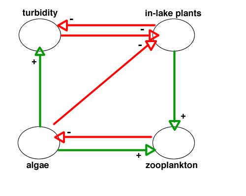
Figure 1. Nodes and interactions in the simplified shallow-lake example. Positive direct effects are denoted with green arrows and a little + sign.
![]() Construct
a logic table for how the state at one time, leads to the outcome at the
next time period. The length of the time period is unspecified at first.
Construct
a logic table for how the state at one time, leads to the outcome at the
next time period. The length of the time period is unspecified at first.
![]() An important consideration
in the selection of the logic is whether multiple factors work together
(requiring an AND statement) or whether each factor on its own could cause
the state (OR statement).
An important consideration
in the selection of the logic is whether multiple factors work together
(requiring an AND statement) or whether each factor on its own could cause
the state (OR statement).
Table lake-example-1.
component state at time step 2 logic statement based on states at time step 1 turbidity(2) algae(1) or not (plants(1)) plants(2) not(algae(1)) OR not(turbidity(1)) algae(2) not(zooplankton(1)) zooplankton(2) algae(1) AND plants(1)
![]() Construct
a input output table and a time series.
Construct
a input output table and a time series.
I will use a shortcut for describing the multiple states of the system. Each possible state consists of the four components in either a high or a low state. This means there are only16 possible combinations of these components. We could right these states out such as turbidity=high, plants =low, algae=high, and zooplankton = low. We could represent each condition as a bit in binary, representing the previous example as 1010. But I chose to represent this binary number in it's decimal equivalent; 1010 base2 = 10 base10. The following table "possible-states" shows all the possible combinations of high and low for each of the four components and the decimal shortcut for that state.
Table "possible-states". The four components are listed in all possible combinations of high and low, 1 and 0. The decimal shortcut is derived by reading the four states as a binary number. For example 0100 base2 = 4 base10.
T P A Z decimal
shorthand0 0 0 0 0 0 0 0 1 1 0 0 1 0 2 0 0 1 1 3 0 1 0 0 4 0 1 0 1 5 0 1 1 0 6 0 1 1 1 7 1 0 0 0 8 1 0 0 1 9 1 0 1 0 10 1 0 1 1 11 1 1 0 0 12 1 1 0 1 13 1 1 1 0 14 1 1 1 1 15
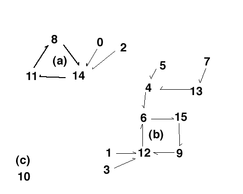
Table lake-scenario-1. A time series of behavior of this system. Time 1 determines time 2. Time 2 determines time 3, etc. The states of the four components are represented in decimal form.
time1 time 2 time3 time4 time5 time6 0 14 11 8 14 11 1 12 6 15 9 12 2 14 11 8 14 11 3 12 6 15 9 12 4 6 15 9 12 6 5 4 6 15 9 12 6 15 9 12 6 15 7 13 4 6 15 9 8 14 11 8 14 11 9 12 6 15 9 12 10 10 10 10 10 10 11 8 14 11 8 14 12 6 15 9 12 6 13 4 6 15 9 12 14 11 8 14 11 8 15 9 12 6 15 9
Scenario1-logic statements
T= algae OR not plants
P = not algae OR not turbidity
A = not zooplankton
Z = algae AND plants
Figure scenario-1-basins. Basins for the logic output. There are three basins/attractors in this particular logic. Basin a is a periodic attractor of the states 8, 14 and 11). Basin b is also a periodic attractor of 6, 15, 9 and 12. Basin c is a point attractor of state 10.
Analysis of these basins and the consequence of switches of logic
scenario 2
change only that Plants depends on not algae AND not turbidity (rather than OR)
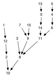
all states go to 10 (turbidity and algae)
| Table "scenario2 logic". It takes upto 5 time steps for all possible initial conditions to end up in state 10; (high turbidity, low plants, high algae, low zooplankton). | Figure "scenario2-basins". There is only one basin in this scenario. All initial conditions lead to state 10. It is interesting that some intial states take five time steps to reach the final state. |
|
T = algae OR not plants P = not algae AND not turbidity A = not zooplankton Z = plants AND algae |
|
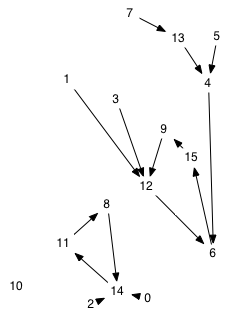
Scenario 3, same as scenario 1 except it takes both algae and an absence of plants to create a high turbidity zone. This results in a more dynamic set of basins than in scenario 2, but none of them (except when you start with no plants and high turbidity) maintain high turbidity.
| Table "scenario3-logic" |
Figure "scenario3-basins" |
T = algae AND not plants P = not algae OR not turbidity A = not zooplankton Z = plants AND algae |
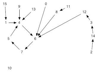 |
Figure shallow-lake-scen3. The basins in this third scenario show how all of these conditions (except high turbidity and algae) lead to a periodic attractor that includes lake plants and clear water.
The analysis of these three scenarios shows that the a slight change in the logic (not the connectivity structure) can result in a very dynamic community, a community that all goes to high turbidity and algae or a community that has a dynamic population structure but maintains clear water.
scenario 1 to scenario 2. Scenario 2 requires that plants will only grow if there is both low algae AND low turbidity. This means there are few conditions that lead to plant growth and hence a domination by algae and turbidity. This shift in logic could be the result of an environmental shift that favors algae over plants (such as slightly deeper water or warmer conditions or more nutrients).
scenario 1 to scenario 3. Scenario 3 requires that turbidity is high when there are both high algae AND no plants. This could come about with a long term shift in conditions that favor plant persistance even in turbid conditions. The basins shows how any condition (except starting with high turbidity and no plants) will eventually lead to plants being part of the system.
scenario 2 to 3. The change from scenario 2 to 3 or vise verse illustrates the hysteresis effect. It requires two changes in the logic. ** expand on this point here with a detailed example, walk through **
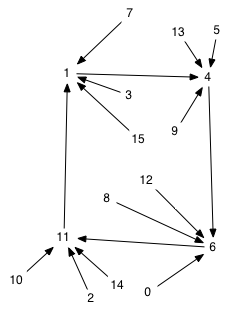
Scenario 4 - simple logic that leads to a periodic attractor.
| Table "scenario 4 logic"
|
Figure "scenario 4 basins". The basin 1,4,6,11 might represent a seasonal pattern of populations in the water. |
T = algae and not zooplankton P = not algae A = not zooplankton Z = algae |
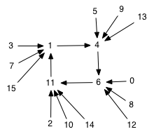 |
table "comparison of logics"
| scenario1 | scenario2 | scenario3 | scenario4 |
T= algae OR not plants P = not algae OR not turbidity A = not zooplankton Z = algae AND plants |
T = algae OR not plants P = not algae AND not turbidity A = not zooplankton Z = plants AND algae |
T = algae AND not plants P = not algae OR not turbidity A = not zooplankton Z = plants AND algae |
T = algae AND not zooplankton P = not algae A = not zooplankton Z = algae |
| 3 basins | all go to 10 | 2 basins | 1 periodic |
scenario 1 to scenario 2 , only change OR to AND for plant logic
Table "comparison of scenario1 to scenario2 for plant column
| dec input |
scen1-plant | scen2-plant | scen1 out | scen 2 out |
| 0 | 1 | 1 | 14 | 14 |
| 1 | 1 | 1 | 12 | 12 |
| 2 | 1 | 0 | 14 | 10 |
| 3 | 1 | 0 | 12 | 8 |
| 4 | 1 | 1 | 6 | 6 |
| 5 | 1 | 1 | 4 | 4 |
| 6 | 1 | 0 | 15 | 11 |
| 7 | 1 | 0 | 13 | 9 |
| 8 | 1 | 0 | 14 | 10 |
| 9 | 1 | 0 | 12 | 8 |
| 10 | 0 | 0 | 10 | 10 |
| 11 | 0 | 0 | 8 | 8 |
| 12 | 1 | 0 | 6 | 2 |
| 13 | 1 | 0 | 4 | 0 |
| 14 | 0 | 0 | 11 | 11 |
| 15 | 0 | 0 | 9 | 9 |
Comparison of a logic change that leads shifts in basin structure and connections.
The states can be arranged on the diagram so that they stay in the same place. Then the logic shift results in rewiring the connections. In the comparison of scenario 1 to scenario 4, this shows that the change in logic results in
| Figure "scenario1-alt" | Figure "scenario4-alt" |
 |
 |
** Replace with an analysis for scenario 2 where state 10 is the final outcome to one of the other scenarios that are "healthier" in the sense that there are more possible states. ***
Model 3: Dynamic Simulation
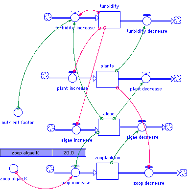
A dynamic simulation of a shallow lake system requires assigning values to all of the initial conditions and rates. In this type of simulation, the system starts from one set of initial conditions and proceeds. In contrast, in the network model above, all possible initial conditions for the four stocks (turbidity, plants, algae and zooplankton) are explored simultaneously.
algae(t) = algae(t - dt) + (algae_increase - algae_decrease) * dt
INIT algae = 20
INFLOWS: algae_increase = 10/turbidity
OUTFLOWS: algae_decrease = .1*zooplankton
plants(t) = plants(t - dt) + (plant_increase - plant_decrease) * dt
INIT plants = 20
INFLOWS: plant_increase = 5/turbidity
OUTFLOWS: plant_decrease = algae/(algae+20)
turbidity(t) = turbidity(t - dt) + (turbidity_increase - turbidity_decrease) * dt
INIT turbidity = 10
INFLOWS: turbidity_increase = if turbidity >300 then 0 else algae*nutrient_factor
OUTFLOWS: turbidity_decrease = plants/(plants+20)
zooplankton(t) = zooplankton(t - dt) + (zoop_increase - zoop_decrease) * dt
INIT zooplankton = 5
INFLOWS: zoop_increase = 10*algae/(algae+zoop_algae_K)
OUTFLOWS: zoop_decrease = 10/(plants +.1)
nutrient_factor = 1
zoop_algae_K = 20
This simulation can be used to explore the sensitivity of the system to different parameters.
exploration 1: sensitivity to the efficiency of zooplanton to eat algae (changing the K)
zooplankton have good efficiency at eating algae (K=10)
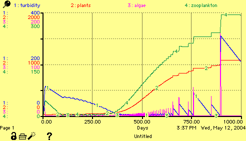
The story on this simulation is:
turbidity and zooplankton are both high (state 9)
zooplankton decrease (state 8)
zooplankton and plants increase (state 5)
and then after time 600 we start seeing additional spikes of algae and turbidity followed by the algae going away and the turbidity dropping more gradually. This would by oscillations between states 15 (all high) and 13 (only algae low)
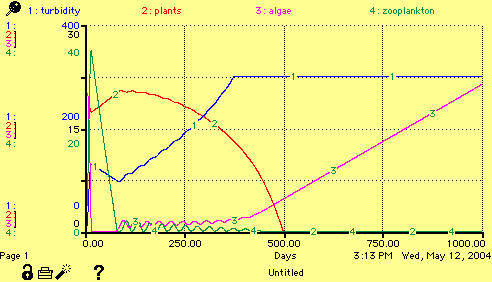
Simulation with the zooplankton being less efficient at low algae concentrations
This simulation demonstrates a very different behavior for what might be considered to be a minor modification of the parameters (i.e. doubling the half-saturation K for zooplankton feeding on algae.
The story on this simulation is:
starting with high zooplankton (state 1)
leads to high plants (state 4)
followed by an increase in turbidity with high plants (state 12)
moving to high turbidity only (state 8)
and then eventually high turbidity and high algae (state 10)
exploration 2:
The question is how to use this model to generate the catastrophe diagrams.
see "multi-stable-states.html"