Interactions with Regression Analysis
Testing and Plotting Simple Slopes
Step 1. Run the
regression analysis, requesting the correlations and covariances of the
regression coefficients using the bcov option.
regression vars=prestige incsq caveinc cwomen
interact
/descriptives=mean stdev n sig corr
/statistics=anova r coeff bcov ses
/dependent=prestige
/method=enter incsq caveinc cwomen interact.
Adding the bcov statement
will provide the following table of estimates of the correlations and
covariances between the regression coefficients in addition to the usual
regression printout. Similar to how the
standard error (Sb) estimates the variability of the regression
coefficient from sample to sample, the values below estimate the association
between regression coefficients b1, b2, etc. from sample
to sample. Correlations are presented
in the top half of the table and covariances are presented in the bottom
half. The diagonal values in the bottom
half of the table are variances.
Highlighted values will be used in next step.
Coefficient
Correlations(a)
öòòòòòòòòòòòòòòòòòòòòòòòûòòòòòòòòòûòòòòòòòòòòûòòòòòòòòòûòòòòòòòòòòø
óModel óINTERACT óCAVEINC óCWOMEN
óINCSQ ó
ùòòòûòòòòòòòòòòûòòòòòòòòôòòòòòòòòòôòòòòòòòòòòôòòòòòòòòòôòòòòòòòòòòú
ó1 óCorrelatioóINTERACTó1.000 ó.369 ó.727 ó.417 ó
ó óns ùòòòòòòòòôòòòòòòòòòôòòòòòòòòòòôòòòòòòòòòôòòòòòòòòòòú
ó ó óCAVEINC ó.369 ó1.000 ó.616
ó-.504 ó
ó ó ùòòòòòòòòôòòòòòòòòòôòòòòòòòòòòôòòòòòòòòòôòòòòòòòòòòú
ó ó óCWOMEN ó.727 ó.616 ó1.000 ó.073 ó
ó ó ùòòòòòòòòôòòòòòòòòòôòòòòòòòòòòôòòòòòòòòòôòòòòòòòòòòú
ó ó óINCSQ ó.417 ó-.504 ó.073 ó1.000 ó
ó ùòòòòòòòòòòôòòòòòòòòôòòòòòòòòòôòòòòòòòòòòôòòòòòòòòòôòòòòòòòòòòú
ó óCovarianceóINTERACTó2.317E-10ó2.282E-09 ó5.487E-07ó1.934E-13 ó
ó ós ùòòòòòòòòôòòòòòòòòòôòòòòòòòòòòôòòòòòòòòòôòòòòòòòòòòú
ó ó óCAVEINC ó2.282E-09ó1.647E-07 ó1.239E-05ó-6.234E-12ó
ó ó ùòòòòòòòòôòòòòòòòòòôòòòòòòòòòòôòòòòòòòòòôòòòòòòòòòòú
ó ó óCWOMEN ó5.487E-07ó1.239E-05 ó2.456E-03ó1.101E-10 ó
ó ó ùòòòòòòòòôòòòòòòòòòôòòòòòòòòòòôòòòòòòòòòôòòòòòòòòòòú
ó ó
óINCSQ ó1.934E-13ó-6.234E-12ó1.101E-10ó9.275E-16 ó
õòòòüòòòòòòòòòòüòòòòòòòòüòòòòòòòòòüòòòòòòòòòòüòòòòòòòòòüòòòòòòòòòò÷
¢
a Dependent
Variable: PRESTIGE
Step 2. Use the
values obtained from the regression analysis in the form below. The choice of X and Z is up to the
researcher and depends on which variable is desired for the X axis. The program used in Step 3 will generate
simple slopes of Y regressed on X at high and low values of Z (one standard
deviation above and below the mean of Z).
In other words, the graph will present the regression line for X
predicting Y twice—once for high values of Z and once for low values of Z.
LABELS: X = CAVEINC
Z= CWOMEN
|
unstandardized b for x |
.005936 |
|
unstandardized b for z |
.312 |
|
unstandardized b for
xz (interaction term) |
.00003525 |
|
mean of x |
.001961 |
|
mean of z |
-.0099804 |
|
std dev for x |
4245.9222 |
|
std dev for z |
31.7249 |
|
std dev for y |
17.204 |
|
constant |
52.173 |
|
variance of x with x ( from bcov matrix) |
.0000001647 |
|
covariance of x with xz (from bcov matrix) |
.000000002282 |
|
variance of xz with
xz (from bcov matrix) |
.0000000002317 |
Step 3. Enter the values
from the form used in Step 2 (in the order on the form, using as many decimal
places as possible) into the following SPSS syntax (electronic copy available
from http://web.pdx.edu/~g3jn/simple.rtf).
DATA LIST
FREE RECORDS=1/ bx bz bxZ MEANX MEANZ
SDX SDZ sdy CONSTANT VARXX VARXXZ COVXZXZ.
COMPUTE
LOWZLOWX=(bx+(bxZ*-SDZ))*(-SDX)+((bz*-SDZ)+CONSTANT).
COMPUTE
LOWZMEDX=(bx+(bxZ*-SDZ))*(MEANX)+((bz*-SDZ)+CONSTANT).
COMPUTE
LOWZHIX=(bx+(bxZ*-SDZ))*(SDX)+((bz*-SDZ)+CONSTANT).
COMPUTE
MEDZLOWX=(bx+(bxZ*MEANZ))*(-SDX)+((bz*MEANZ)+CONSTANT).
COMPUTE
MEDZMEDX=(bx+(bxZ*MEANZ))*(MEANX)+((bz*MEANZ)+CONSTANT).
COMPUTE
MEDZHIX=(bx+(bxZ*MEANZ))*(SDX)+((bz*MEANZ)+CONSTANT).
COMPUTE
HIZLOWX=(bx+(bxZ*SDZ))*(-SDX)+((bz*SDZ)+CONSTANT).
COMPUTE
HIZMEDX=(bx+(bxZ*SDZ))*(MEANX)+((bz*SDZ)+CONSTANT).
COMPUTE
HIZHIX=(bx+(bxZ*SDZ))*(SDX)+((bz*SDZ)+CONSTANT).
COMPUTE
LOWZSLOP=bx+(bxZ*-SDZ).
COMPUTE
MEDZSLOP=bx+(bxZ*MEANZ).
COMPUTE
HIZSLOP=bx+(bxZ*SDZ).
COMPUTE
ERRSLP1=SQRT(VARXX+(2*(-SDZ)*(VARXXZ))+(-SDZ*-SDZ)*COVXZXZ).
COMPUTE
ERRSLP2=SQRT(VARXX+(2*(MEANZ)*(VARXXZ))+(MEANZ*MEANZ)*COVXZXZ).
COMPUTE
ERRSLP3=SQRT(VARXX+(2*(SDZ)*(VARXXZ))+(SDZ*SDZ)*COVXZXZ).
COMPUTE STANSLP1=LOWZSLOP*(SDX/SDY).
COMPUTE STANSLP2=MEDZSLOP*(SDX/SDY).
COMPUTE STANSLP3=HIZSLOP*(SDX/SDY).
COMPUTE TSLOPE1=LOWZSLOP/ERRSLP1.
COMPUTE TSLOPE2=MEDZSLOP/ERRSLP2.
COMPUTE TSLOPE3=HIZSLOP/ERRSLP3.
BEGIN DATA.
.005936 .312 .00003525
.001961 -.0099804 4245.9222 31.7249 17.204 52.173 .0000001647
.000000002282 .0000000002317
END DATA.
LIST VARIABLES=LOWZLOWX LOWZHIX HIZLOWX HIZHIX.
LIST VARS=LOWZSLOP HIZSLOP
ERRSLP1 ERRSLP3 STANSLP1 STANSLP3.
LIST
VARS=TSLOPE1 TSLOPE3.
Note:
BX, BZ, and BXZ are the unstandardized regression coefficients for the first
predictor variable, the second predictor variable, and the interaction term,
respectively. MEANX and MEANZ are the
means, and SDX, SDZ, and SDY are the standard deviations. CONSTANT is the
constant or intercept value. VARXX is
the estimated variance of the regression coefficient for the continuous
predictor. VARXZXZ is the estimated
variance of the regression coefficient for the interaction term (from the
diagonal of the bcov matrix. COVXXZ is
the estimated covariance between the first predictor slope (b for X variable) and
the interaction term slope (b for XZ). The program prints out the plot points
for plotting two simple slope regression lines (LOWZLOWX LOWZHIX, HIZLOWX,
HIZHIX), unstandardized slope estimates (LOWZSLOP, HIZSLOP), their standard
errors (ERRSLP1,ERRSLP3), standardized slopes (STANSLP1, STANSLP3), and the
t-tests for the coefficients (TSLOPE1, TSLOPE3). To test simple slopes when the Z predictor is dummy coded:
replace –SDX with 0 and SDX with 1 in the first set of compute statements. To test simple slopes when an unweighted
effect code is used: replace –SDX with –1 and SDX with 1 in the first set of
compute statements. To test simple
slopes with weighted effect codes: replace –SDX with –P1/Pother
and SDX with 1. P1 is the
proportion of the sample coded 1 under effect or dummy coding, and Pother
is the proportion in the other group (coded 0 in dummy coding or –1 in effect
coding).
Step 4. Below is the
printout obtained from the program in Step 3.
It contains the simple slopes for 1 standard deviation above and below
the mean on cwomen (LOWSLOP and HISLOP, respectively). The plot points (LOWZLOWX,
LOWZMEDX, LOWZHIX, HIZLOWX, HIZMEDX, HIZHIX) can be used to plot simple slopes
by hand or with Excel.
List
LOWZLOWX LOWZHIX
HIZLOWX HIZHIX
21.82 62.73
32.12 92.02
Number of cases
read: 1 Number of cases listed:
1
List
The variables are
listed in the following order:
LINE 1: LOWZSLOP HIZSLOP ERRSLP1 ERRSLP3
STANSLP1
LINE 2: STANSLP3
LOWZSLOP: .00 .01
.00 .00 1.19
STANSLP3: 1.74
Number of cases
read: 1 Number of cases listed:
1
List
TSLOPE1 TSLOPE3
9.58 9.58
Number of cases read:
1 Number of cases listed: 1
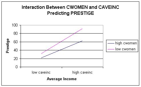
Step 5. Plot the
interaction. Below is a plot generated
using Excel for the prestige data example.
