Lab 3 Part 1: Processing LiDAR Data

Introduction

This lab has four separate tasks that will introduce you to the process of converting raw LiDAR returns to useable GIS data. Task 1 involves using ENVI LiDAR to perform feature extraction on LiDAR data. Tasks 2 and 3 discuss the basic steps of processing LiDAR data in ArcGIS. Task 4 deals with 3D visualization of LiDAR data.

Spend some time exploring the functionality introduced in this lab – it’s the best way to get acquainted with both the software and the data. Use the help system to learn about the different options. If you have a question, ask.

Type the answers to all the questions at the end of each tasks, attach any documents and maps (or images) that are requested.

The files used in Lab 3 (both Parts 1 & 2) are in the I:\Students\Instructors\Geoffrey_Duh\GEOG4593\Lab3 folder. Please copy lab data to your local workspace before you start the lab.

You can find the ENVI LiDAR program from ENVI 5.4's Toolbox. First, you start ENVI 5.4. Then find the "Launch ENVI LiDAR" tool in the Toolbox. Double-click on the tool to launch it.

Task 1 – LiDAR Feature Extraction in ENVI

Instructions

Complete the exercises of ENVI LiDAR tutorial. In the task, you will use ENVI LiDAR to view and extract features from LiDAR raw data. Depending on the density of the raw LiDAR data points, one can extract various landscape features from LiDAR, including DEM, DSM, buildings (rooftop), trees (canopy), power lines, or even power poles. The software uses various algorithms to recognize these landscape features based on the 3D spatial patterns of LiDAR point cloud. Some of the processes might take a significant amount of time to complete. Please be patient!

After completing the tutorial using the tutorial data (DataSample.las), repeat the same process with the additional data set (45122D7103_clip.las) that you find in the lab folder. The spatial reference for 45122D7103_clip.las is State Plane, Oregon North (FIPS3601), International Feet. You will need to use the "Advanced" option to set the projection to State Plane. The datum is NAD83 (Washington-Oregon HPGN). HPGN stands for High Precision Geodetic Network and is synonymous to HARN (High Accuracy Reference Network) that is used in ArcGIS. When both las files are processed, examine how well the features were extracted from each. Capture a screenshot of the 3D Google Earth view of the buildings derived from 45122D7103_clip.las. Answer the questions below.

Questions

1.      When selecting a display area from the ENVI navigate window, ENVI shows the point density information in the operations log area (at the bottom of the screen).What are the average point densities (point/m²) for DataSample.las and for 45122D7103_clip.las?

Las file	Average point density (points/m2)
DataSample.las
45122D7103_clip.las

 

2.      What areas (i.e., land cover types) on each las data files have the highest average point densities? What are the point densities?

Las file	Cover Type(s)	Highest point density (points/m2)
DataSample.las
45122D7103_clip.las

 

3.      What areas (i.e., land cover types) on both las data files have the lowest average point density? What are the point densities?

Las file	Cover Type(s)	Lowest point density (points/m2)
DataSample.las
45122D7103_clip.las

 

4.      Where is the area for the 45122D7103_clip.las data? Insert a screenshot of the 3D buildings on Google Earth here.

 

Task 2 – Import Preprocessed LiDAR Data

Instructions

This task is to import a preprocessed (i.e., filtered) LiDAR data points into a GIS dataset that you can manipulate in your GIS application (in this case, ArcGIS). The goal of this process is to generate digital elevation models stored as raster grids. The dataset used in this task covers a different area from the dataset used in Task 1. Also, the data have been converted to x, y, z values stored in Dbase dbf format. This is an example of how you could import LiDAR points into ArcGIS. When working with GIS data, you should pay attention to the unit (e.g., feet, meters, square meters, etc) of the data you are working with.

1. Add the "LiDAR_Returns_Bare_Earth_0503.dbf" file to ArcMap and view its content. These are the "bare earth" (surface) LiDAR returns for a small area of Portland. The table contains the X/Y/Z coordinates of the returns in Stateplane feet. The X attribute is X_COORD, the Y attribute is Y_COORD, and the Z value (or elevation) is Z_VALUE.

2. Open ArcMap. Go to File/Add data – Add XY data. Browse to the bare earth dbf. Make sure the specified X Field, Y Field and Z Field are correct. You will also need to define the projection of the data. Click the Edit button, click Select to select a predefined coordinate system, and browse to the correct "projected" coordinate system. Here’s the details:

 

Stateplane projection: NAD 1983 HARN (Feet, Intl and US), Oregon North FIPS Zone 3601, International feet

 

3. Click the OK button. The points will be added to the map (this may take a few seconds). Turn on the layer (it will take a minute or two to draw). This is an ArcGIS "event table" layer. Zoom in to the layer and use the Identify tool to click on a few points. An event table layer is a temporary, non-permanent representation of geographic data from coordinates defined in a table. It will persist with the MXD document (meaning if you save the ArcMap document you will save the layer in it). However, it is tied to the original DBASE table, so you cannot change the location of or remove the original table. You can create permanent GIS data from an event table layer by right-clicking the layer and selecting Data – Export Data. You don’t need to use permanent point layers for this task, but you will use them in a later task. Follow the steps above to create permanent layer files for both LiDAR dataset.

4. Repeat steps 1 through 3 for the "first return" LiDAR coordinates in the "LiDAR_Returns_First_Return_0503.dbf" in the same directory as the bare earth returns. Note: there are more points in this dataset – it will take longer to draw.

Questions

1.      How many points are in the "first return" and "bare earth" dataset? What are the estimated average numbers of points per square meter for each dataset? What are the estimated point spacing (in meters and in feet)? Use the table below to answer this question (Hint: The area is rectangular. Make sure you get the correct areal units.)

 

2. Zoom in to a relatively small area and compare the bare earth returns with the first returns. Many of the bare earth returns are also in the first return dataset. Why?

 

Task 3 – Create a TIN and DEM From the LiDAR Returns

Instructions

The second task is to convert the LiDAR returns into a triangulate irregular network (TIN) model and then into a raster "digital elevation model" (DEM) of the surface using the bare earth LiDAR returns. The DEM is usually the final representation of the surface derived from LiDAR points. The raster format is a much more efficient way of storing the large, complex elevation models derived from LiDAR data (the TIN is most often discarded after the DEM is created). Again, there are many ways to do this, and some offer you much more control over the resulting triangulation than others. This is an example of how you would create a TIN and DEM with the standard ArcGIS 3D Analyst Tools. Note that the next few tasks will be performed on the bare earth returns only.

1. Open ArcMap if is not already open. Make sure the 3D Analyst extension is turned on.

2. Turn on the 3DAnalyst toolbar.

3. Search for and start the Create TIN tool. Set the "LiDAR_Returns_Bare_Earth_0503 Events" as the input feature class.

4. Set the Height source to Z_Value. The Z_Value is the elevation of each point above-sea-level. We are creating this TIN from "mass points". Leave the Tag value field as "<None>".

5. Specify a file location and name for the output TIN. Because the output is in ArcInfo coverage format, the name must be 13 characters or less. You may want to indicate that this is the bare earth TIN in the file name (e.g., tin_be). Set the spatial reference the same as the input LiDAR data. Since we don't have any breaklines, the "Constrained Delaunay" option doesn't have any effect on the process.

6. Click OK to create the TIN. This WILL take a while. Zoom in to a smaller area and explore the model (smaller areas draw much faster). Right click on the layer and select Properties. Go to the Symbology tab, and press the Add button. Add a few different renderers to explore the different TIN symbolization options.

7. Start the TIN to Raster tool. Specify the bare earth TIN you created as the Input TIN. Set output data type as FLOAT, method as LINEAR, and sampling distance to "CELLSIZE 5." Leave Z Factor as 1 (this is the amount of vertical exaggeration). Specify a file location and name for the output raster image. Because the output is in ArcInfo GRID format, the name must be 13 characters or less. You may want to indicate that this is the bare earth DEM in the file name (e.g., dem_be).

8. Click OK to create the DEM. When complete, zoom out to the full extent of the DEM. Right click on the layer and select Properties. Go to the Symbology tab, and explore the different symbolization and classification options.

9. Repeat steps in Tasks 2 and 3 to convert the LiDAR_Returns_First_Return _0503.dbf to a DSM (e.g., dsm_fr).

Questions

1. What are the maximum and minimum elevation values in the DEM and in the TIN model? Why are the values in the DEM different from those in the TIN model?

2. You specified a cell size of "5" when creating the DEM and DSM. What does this value represent? Why is "5" an appropriate value for this LiDAR data? (Hint: You need to list the point spacing values for the first and last return data.)

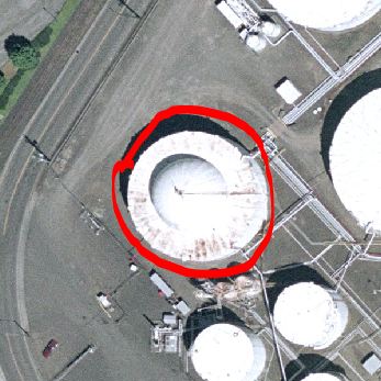
3. Visually compare the bare earth DEM and the first return DSM. What is the height of the "domed" structure just west of the storage tanks?

 

Task 4 – Visualizing the Data in 3D

Instructions

This task is to visualize the data you have created so far in 3D. We will use ArcGIS’s ArcScene for this task. It’s not the best 3D visualization software, but it (usually) gets the job done.

1. Save your MXD and close ArcMap.

2. Open ArcScene (in the Windows Start menu under ArcGIS).

3. Add the bare-earth DEM created in Task 2.

4. Right-click on the layer, select Properties, then select the Base Heights tab. Click on the Floating on a custom surface option, and select the DEM from the drop-down menu. This will render the DEM in 3D using the elevation values from the raster pixels.

5. Click Raster Resolution and enter 10 into Cellsize X and Cellsize Y. This is the resolution to which ArcScene will generalize the DEM (to make it draw faster). If you wanted the DEM to render at its full resolution, you would enter 5 for each value.

6. Click on the Rendering tab. Under Effects, check on Shade areal features relative to scene’s light position. Also, drag the Quality enhancement slider bar a bit to the right, so that the slider sits about 2/3 of the way to "high" (to improve the quality of the rendering).

7. Click the Symbology tab. Select a more colorful Color Ramp.

8. Click OK.

9. Repeat steps 1 through 8 with the first return DSM.

Questions

1. Note that the model has some irregularities on the southern edge. What are some possible ways to remove these kinds of edge issues when generating an elevation model?

2. Play around with the Raster Resolution layer property (in the Base Heights tab). Set it to the maximum resolution (5). For which model does it make the most difference visually? Why?

3. Where is this area in Portland? (Hint: Use RLIS data on the I drive to figure it out.)

Export a view of the full first return DSM from ArcScene (File – Export Scene – 2D) as a .emf file. You can then insert the .emf to a Word document. Print out a copy and turn it in with your lab report.