Lab 3 Part 2: Using LiDAR-Derived Terrain Data

Introduction

This lab has four separate tasks that will introduce you to working with LiDAR-derived elevation models. Tasks 1 and 2 uses the LiDAR DEM and DSM to determine (and visualize) surface feature heights. Task 3 introduces the concept of using other remotely-sensed imagery and data to classify the height image. Task 4 deals with the extraction of summary statistics from the LiDAR data.

Type the answers to all the questions at the end of each task, attach any documents and maps that are requested.

The files used in this lab are the same as those used in Lab 3 Part 1. They are in the I:\Students\Instructors\Geoffrey_Duh\GEOG4593\Lab3 folder.

Task 1 - Creating a Height Image

Instructions

The first task is to compare the bare earth return digital elevation model (DEM) with the first return digital surface model (DSM) to derive the heights of features on the ground. We'll use ArcGIS' Spatial Analyst to do the comparison, though the basic process is more or less consistent regardless of the software used.

Note: We've also provided 2005 6" resolution aerial photos for this area for your use in this lab. You can find them in the 2005_Aerials folder and add them to your ArcMap document for visual reference.

1.      Open ArcMap. Make sure the Spatial Analyst extension is turned on (Customize menu - Extensions - check on Spatial Analyst).

2.      Add both the DEM and the DSM grids that you created in Part 1 of Lab 3 to the view. If you saved your work from Part 1 in an MXD document, you open it to retrieve your data. (Note: for the purposes of these exercises, the DEM and DSM grids created in Part 1 will be referred to as "dem_be" and "dsm_fr". Substitute your own file names where appropriate.)

3.      Search for Raster Calculator and start it. The Raster Calculator, despite its name and appearance, is much more than a calculator. It's a powerful analysis tool - you can access many Spatial Analyst function using the correct syntax, build complex expressions, and do conditional queries. (For more information, press the Tool Help button and follow the help links).

4.      To create the feature height image, subtract the DEM from the DSM by typing the following expression into the calculator (you can add the appropriate layer names by double-clicking them in the Layers box; you can add mathematical expressions and numbers by pressing the buttons):

"dsm_fr" - "dem_be"

Name the output raster "dsm_dem", that is dsm minus dem, and save it to your workspace. Press OK to verify the expression and create the output raster.

5.      Note the minimum and maximum values of the height grid. The -207 minimum value is obviously an error in the data (there are always a few, but they usually do not have a significant impact on the elevation model if the LiDAR data was pre-processed correctly by the vendor). Let's create another raster that shows only the negative values so we can evaluate them. We'll use the conditional function con, which uses the following syntax:

con({test condition}, {true expression}, {false expression})

This is an extremely useful function. For our purposes, let's reclassify all values in the height image into 2 classes (0 and 1). Open the Raster Calculator again and type or build in the following expression:

Con("dsm_dem" < 0, 1, 0)

Name the output raster "neg_fh" and save it to your workspace. Press OK. The output raster will be added to the table of contents.

6.      We know that negative height values are not possible. Let's create the final "Feat_Height" height image by forcing all negative values to evaluate as 0. Open the Raster Calculator again and type, build, or copy in the following expression:

Con(("dsm_fr" - "dem_be") < 0, 0, "dsm_fr" - "dem_be")

Name the output raster "Feat_Height". Press OK.

Questions

1.      Refer to the reclassified height image we created ("neg_fh"). Based on the conditional equation we constructed in step 5, what do the "0" value pixels represent? What do the "1" value pixels represent?

2.      Use the reclassified height image ("neg_fh") and the color aerial photos to examine where the negative values are located. Ignoring edge effect issues, which is a result of the DEM and DSM models being a slightly different size, is there anything consistent about where the negative values are located? Use the Identify tool to click on some of the negative value pixels in the original height image ("dsm_dem") created in step 4. Do the values tend to be large or small? What are some possible reasons that there are negative values?

3.      All the tanks in the tank farm in the eastern portion of the image area are roughly the same height. What is that height?

4.      What is the height of the tallest feature in the image area? What is that feature likely to be?

Task 2 - Visualizing the Height Image in 3D

Instructions

The second task is to visualize the height image you have created so far in 3D. These steps are essentially identical to those in Task 4 of Part 1, but I'll repeat them here for your reference.

1.      Save your MXD.

2.      Open ArcScene.

3.      Add the "Feat_Height" height image created in Task 1.

4.      Right-click on the layer, select Properties, then select the Base Heights tab. Click on the Floating on a custom surface option, and select the DEM from the drop-down menu. This will render the DEM in 3D using the values from the raster pixels.

5.      Click Raster Resolution and enter 5 into Cellsize X and Cellsize Y. We will render the data at its full resolution.

6.      Click on the Rendering tab. Under Effects, check on Shade areal features relative to scene's light position. Also, drag the Quality enhancement slider bar a bit to the right, so that the slider sits about 2/3 of the way to "high" (to improve the quality of the rendering).

7.      Click the Symbology tab. Select a more colorful Color Ramp.

8.      Click OK.

Questions

1.      Compare the Feat_Height model to the DSM ("fr_dsm") created in Task 3 of Part 1. Explain the difference.

2.      Export a view of the rendered height image from ArcScene (File - Export Scene - 2D) to an emf file and insert the emf file into your MS Word document. Print out a copy and turn it in with your lab.

Task 3 - Classifying the Height Image

Instructions

The third task is to classify the height image into a "canopy heights" image using a 2002 multispectral classification for the same area. The purpose of this exercise is to illustrate how different image datasets can be compared and combined to add value to the original information.

1.      Open ArcMap if is not already open. Add the 2002_ms_classification dataset in the 2002_MS_Data folder to the MXD. Right-click on the layer, select Properties, click on the Symbology tab, the select "Unique Values" in the Show box. Click on the Display tab and set Transparent to 50%. Press OK. This is a 1-meter classification showing 4 general land cover classes - vegetation, impervious surfaces, loose surfaces (dirt), and water.

2. Add the raster dataset "Feat_Height" to ArcMap. Open the Raster Calculator. We'll use the following equation to classify the height image ("Feat_Height"):

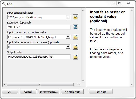
It seems that the Raster Calculator tool won’t be able to produce a correct result on the following calculation. Please use the CON tool in Arctoolbox to complete the step. Click here for a screenshot of the CON tool.

Con("2002_ms_classification.img" == 4, "Feat_Height", 0)

Name the output raster as "canopy_hgt". Press OK. Note that "4" is the value of the vegetation class in the multispectral image.

3.      Right-click on the "canopy_hgt" layer, select Properties, click the Symbology tab, select "Classified" in the Show box, and select an more appropriate color ramp (light green to dark green, for example). Then click on the Classify button, click the Exclusion button, click on the Value tab if necessary, and type "0" into the Excluded values box. Press OK three times to dismiss all dialog windows.

Questions

1.      Explain (in no more than a sentence or two) what this canopy height classification has produced? Why would this image be useful?

2.      The "vegetation" class in the multispectral image represents all vegetation types (trees, shrubs, grasses). If you wanted to reclassify the canopy height image you created in this task to attempt to isolate trees, what is one possible (and common) way to do it? Refer to Task 1, step 5 or 6, and write a conditional expression using the con function that would accomplish this (Hint: you are trying to isolate trees from shrubs and grasses).

3.      Luckily for you, the vegetation has already been classified into "tree canopy" and "non tree-canopy vegetation". You can view the "2002_ms_canopy_classification" image in the 2002_MS_Data folder. Using this image, and referring to step 2 above, create a tree canopy height classification image using the Raster Calculator. Name it "tree_height". The value of the "canopy vegetation" class is "2". What are the minimum and maximum values of the resulting tree canopy height image?

Task 4 - Summarizing Height Information by Geographic Area

Instructions

The final task will be to generate summary statistics from for a set of four 100'-radius sample plots using the classified tree canopy height image. The purpose of this exercise is to illustrate how one might determine the maximum, minimum, or average height for a set of predefined geographic areas (such as sample plots, building footprints, neighborhood, etc.)

1.      Add the "Sample_Plots" shapefile in your lab folder to your ArcMap document.

2.      For the purpose of this exercise, we are only interested in trees above 20' in height. We also want to make sure that all values less than 20' are set to NULL (a.k.a. NoData), rather than 0, so that they will not be considered in our summary statistics for each sample plot (0 values would be factored into the mean calculation, for example). We'll use the "SetNull" function, which has the following syntax:

setnull({"null" condition}, {output value image name})

If the "null" condition evaluates as "true", the specified grid values will be calculated as null. Open the Raster Calculator again and type in or build the following expression to reclassify our tree height image:

SetNull("tree_height"  < 20, "tree_height")

Name the output raster as "tree_gt20". Press OK.

3.      We can now create summary statistics for each of the sample plots. Search for the "Zonal Statistics as Table" tool and start it. Specify the "Sample_Plots" shapefile as the zone data. For the Zone field, select "Plot_ID". Specify "tree_gt20" as the Value raster. Save output as "plot_stats" in your lab folder. Check on Ignore NoData in calculations. Use ALL as the statistics type. Press OK to execute the tool. When done, join the table to the sample plot shapefile using "Plot_ID" as the key.

Questions

1.      Which sample plot has the tallest tree? Which plot has the tallest trees on average? Complete the table below to find your answers.

 

2.      We know each of these sample plots has a 100' radius. What is the area of each plot? Roughly how many LiDAR pixels should be in each plot (given the resolution our elevation models)? The "Count" field in the summary table indicates how many "canopy" pixels with a height of more than 20' are in each plot. What percentage of each plot is covered in canopy above 20' in height?

 

Optionally, you can use the same summary technique to calculate the maximum, minimum, and average slope and elevation for each plot. You may find relationships between the tree condition and the terrain properties.