Lab 3 Part 1: Processing LiDAR Data

Due by Oct 29

Introduction

This lab has five separate tasks that will introduce you to the process of converting raw LiDAR returns to useable GIS data. Tasks 1 through 3 discuss the basic steps of processing LiDAR data in ArcGIS. Task 4 introduces ModelBuilder as a way to automate the processing. Task 5 deals with 3D visualization of LiDAR data.

Spend some exploring the functionality introduced in this lab – it’s the best way to get acquainted with both the software and the data. Use the help system to learn about the different options. If you have a question, ask. This is brand new data for Portland – take a bit of time to explore it.

Type the answers to all the questions at the end of each task, attach any documents and maps that are requested.

The files used in Lab 3 (both Parts 1 & 2) are in the I:\Students\Instructors\Geoffrey_Duh\GEOG4593\Lab3 folder. You are only allowed to put data in the C:\Users folder on the computers in CH469 or CH475. You can use your odin ID or your name to create a working folder in C:\Users so that your data won’t get mixed with other students’. If you want to access your working folder from other computers on campus, please follow the instructions on this page . Then create a folder for Lab 3.

Task 1 – import raw LiDAR data

Instructions

The first task is to import the “raw” LiDAR data points into a GIS dataset that you can manipulate in your GIS application (in this case, ArcGIS). There are many ways to do this, some more efficient than others. This is an example of how you would import LiDAR points into ArcGIS.

1. Double-click the “LiDAR_Returns_Bare_Earth_0503.dbf” file to view its content in MS Excel. These are the “bare earth” (surface) LiDAR returns for a small area of Portland.

2. Note that if you will only see the first 65,000 or so records (which is its limit). Also note that Excel does not tell you this (be wary of working with LiDAR data in Excel). These are the X/Y/Z coordinates of the returns in Stateplane feet. The X attribute is X_COORD, the Y attribute is Y_COORD, and the Z value (or elevation) is Z_VALUE. Close the file.

3. Open ArcMap. Go to Tools – Add XY data. Browse to the bare earth dbf. Make sure the specified X Field and Y Field are correct. You will also need to define the projection of the data. Click the Edit button, click Select to select a predefined coordinate system, and browse to the correct “projected” coordinate system. Here’s the details:

Stateplane projection: NAD 1983 HARN (Feet, Intl and US), Oregon North FIPS Zone 3601, International feet

4. Click the OK button. The points will be added to the map (this may take a few seconds). Turn on the layer (it will take a minute or two to draw). This is an ArcGIS “event table” layer. Zoom in to the layer and use the Identify tool to click on a few points. An event table layer is a temporary, non-permanent representation of geographic data from coordinates defined in a table. It will persist with the MXD document (meaning if you save the ArcMap document you will save the layer in it). However, it is tied to the original DBASE table, so you cannot change the location of or remove the original table. You can create permanent GIS data from an event table layer by right-clicking the layer and selecting Data – Export Data. You don’t need to use permanent point layers for this task, but you will use them in a later task. Follow the steps above to create permanent layer files for both LiDAR dataset.

5. Repeat steps 1 through 4 for the “first return” LiDAR coordinates in the “LiDAR_Returns_First_Return_0503.dbf” in the same directory as the bare earth returns. Note: there are more points in this dataset – it will take longer to draw.

Questions

1. How many points are in the “first return” dataset? What is the estimated average number of points per square meter? (Hint: The area is rectangular. Be aware of your units.)

2. Explain some possible reasons that there are areas in the bare earth dataset that have no returns (Hint: Use the aerial photos in the 2005_Aerials to find clues).

3. Zoom in to a relatively small area and compare the bare earth returns with the first returns. Many of the bare earth returns are also in the first return dataset. Why?

Task 2 – create a TIN and DEM from the LiDAR returns

Instructions

The second task is to convert the LiDAR returns into a triangulate irregular network (TIN) model and then into a raster “digital elevation model” (DEM) of the surface using the bare earth LiDAR returns. The DEM is usually the final representation of the surface derived from LiDAR points. The raster format is a much more efficient way of storing the large, complex elevation models derived from LiDAR data (the TIN is most often discarded after the DEM is created). Again, there are many ways to do this, and some offer you much more control over the resulting triangulation than others. This is an example of how you would create a TIN and DEM with the standard ArcGIS 3D Analyst Tools. Note that the next few tasks will be performed on the bare earth returns only.

1. Open ArcMap if is not already open. Make sure the 3D Analyst extension is turned on (Tools menu – Extensions – check on 3D Analyst).

2. Turn on the 3DAnalyst toolbar.

3. From the toolbar, select 3D Analyst – Create/Modify TIN – Create TIN from Features.

4. Check the box next to the “LiDAR_Returns_Bare_Earth_0503 Events” in the Layers window.

5. Set the Height source to Z_Value. The Z_Value is the elevation of each point above-sea-level. We are creating this TIN from “mass points”. Leave the Tag value field as “<None>”.

6. Specify a file location and name for the output TIN. Because the output is in ArcInfo coverage format, the name must be 13 characters or less. You may want to indicate that this is the bare earth TIN in the file name (e.g., tin_be).

1. Click OK to create the TIN. This WILL take a while. Zoom in to a smaller area and explore the model (smaller areas draw much faster). Right click on the layer and select Properties. Go to the Symbology tab, and press the Add button. Add a few different renderers to explore the different TIN symbolization options.

2. From the toolbar, select 3D Analyst – Convert – Create TIN to Raster.

3. Specify the bare earth TIN you created as the Input TIN. Click the Attribute drop down. Note that there are several options for raster data that you can create from the TIN. Select “Elevation”. Leave Z Factor as 1 (this is the amount of vertical exaggeration). For cell size, enter “5”.

4. Specify a file location and name for the output raster image. Because the output is in ArcInfo GRID format, the name must be 13 characters or less. You may want to indicate that this is the bare earth DEM in the file name (e.g., dem_be).

5. Click OK to create the DEM. When complete, zoom out to the full extent of the DEM. Right click on the layer and select Properties. Go to the Symbology tab, and explore the different symbolization and classification options.

Questions

1. What are the maximum and minimum elevation values in the DEM? Why are they different from the TIN model?

2. You specified a cell size of “5”. What does this value represent? Why is “5” an appropriate value for this LiDAR data (refer to Task 1, question 1)? If the answer to Task 1, question 1 was “8” points per square meter, what would be an appropriate minimum cell size?

Task 3 – create additional datasets from the DEM

Instructions

The fourth task is to use the DEM you have created to generate some additional datasets. We’ll create a hillshade and some contours, which are commonly generated from elevation models.

1. Make sure the 3DAnalyst toolbar is visible.

2. From the toolbar, select 3D Analyst – Surface Analysis – Hillshade.

3. Specify the DEM you created in Task 2 as the Input surface. Check on the Model Shadows check box. Accept the default Azimuth, Altitude and Z Factor. Specify an Output Cell Size of “5”.

4. You have the option of creating the hillshade as a temporary file or as a permanent raster dataset. To create a permanent dataset, browse to the output directory and specify a file name (13 characters or less). Temporary data will not be written to disk, only added to the ArcMap document (you can always make it “permanent” later by right-clicking the layer and selecting Make Permanent.)

5. From the 3D Analyst toolbar, select 3D Analyst – Surface Analysis – Contour.

6. Specify the DEM you created in Task 2 as the Input surface. Enter “5” as the Contour interval. Leave all other settings at the default value.

7. Specify a file location and name for the output contours. There is no limit on file name because the output is in shapefile format. You may want to indicate that these are the bare earth contours, and the contour interval, in the file name (e.g., 5ft_contours_bare_earth).

Questions

1. You specified an “azimuth” and “altitude” when creating the hillshade. Explain what each of these parameters represents. What is unusual about these values? What would the values be for October 23, 2008, at noon (Hint: go to http://aa.usno.navy.mil/data/docs/AltAz.php). Create another hillshade using the 10/23/2008 values. Which of the hillshades do you prefer and why?

2. Take a look at the hillshade and the contours. Describe some of the surface features (in layman’s terms) that are likely present in this area based on your observations.

Task 4 – automating LiDAR data processing

Instructions

The fifth task is to automate Tasks 2 and 3 into a single process that you will use to process the first return LiDAR points into a TIN, “digital surface model” (DSM), hillshade and contours. There are several ways to automate processing within ArcGIS using scripting (Visual Basic, C++, Python, and AML) or “models”. We’ll create a model using ArcGIS’s ModelBuilder to process our data.

Note about Task 4: ModelBuilder can be frustrating. Make sure you use the online help to learn more about ModelBuilder’s features. If you cannot get your model to work, talk to your instructor. If that’s not an option, process the first return manually using the steps in Tasks 2 and 3, and answer whatever questions you can below. It’s less important that it works than you get a sense of what’s possible to automate.

1. Open ArcCatalog.

2. Browse to a directory location where you have write access (e.g., c:/users). Right click in this directory, select New – Toolbox, then type “LiDAR Tools” as the name for your custom toolbox.

3. Open ArcToolbox in ArcMap.

4. There are two ways you can add your custom toolbox to ArcMap. In ArcToolbox, right click the “ArcToolbox” folder and select Add Toolbox, then browse to the “LiDAR Tools” toolbox you just created. Or you can simply drag and drop the “LiDAR Tools” toolbox from ArcCatalog to ArcToolbox.

5. Right-click the LiDAR Tools toolbox, and select New – Model.

6. The ModelBuilder window should open. Click on the Model menu, select Model Properties, click on the General tab, and specify a name and label for your model (e.g., “ProcessLiDAR”). They can be the same but the name of the model can not have spaces or underscores. Save the model. (Note: by default, the model will be saved to C:\Documents and Settings\{user name}\Application Data\ESRI\ArcToolbox\My Toolboxes.)

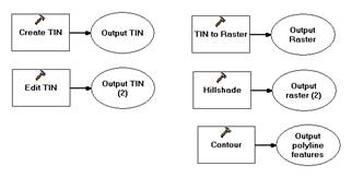
7. Open the 3D Analyst toolbox in ArcToolbox. Open the TIN Creation folder. Click and drag the Create TIN tool from ArcToolbox to your new spatial model.

8. Open the TIN Creation folder in the 3D Analyst toolbox. Click and drag the Edit TIN tool from ArcToolbox to your new spatial model.

9. Open the Conversion folder in the 3D Analyst toolbox. Click and drag the TIN to Raster tool from ArcToolbox to your new spatial model.

10. Open the Raster Surface folder in the 3D Analyst toolbox. Click and drag the Hillshade tool from ArcToolbox to your new spatial model. Also click and drag the Contour tool from ArcToolbox to your new spatial model.

Your model should now look something like this:

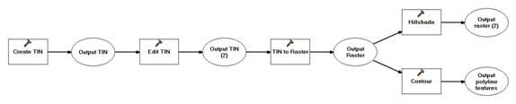
11. Use the “connect” tool (2^nd from right on the toolbar, the cursor turns to a little magic wand) to connect the following:

a. Output TIN to Edit TIN

b. Output TIN (2) to TIN to Raster

c. Output Raster to BOTH Hillshade and Contour

Click the “select” tool on the ModelBuilder toolbar and select the individual pieces and move them into some kind of logical order (you can also press the button with 4 squares, 2 blue, 2 green, to auto-arrange your model). Your model should now look something like this:

12. Right-click the Create TIN box and select Make Variable – From Parameter – Spatial Reference (this is the projection information that you will provide when you run the model). You can set the parameters of a tool with variables or by directly typing the values on the tool’s dialog. To open a tool’s dialog window, just double-click the tool in ModelBuilder.

13. Right-click on the Edit TIN box and select Make Variable – From Parameter – Input Feature Class (this is the layer that you will specify to be processed when you run the model).

14. Right-click on the Contour box and select Make Variable – From Parameter – Contour interval (this is the contour interval in feet that you will specify when you run the model).

15. Double-click the TIN to Raster box. Under Sampling Distance, select CELLSIZE, and change the number to “5” (so that it reads “CELLSIZE 5”). This is the resolution of your output raster data. Click OK to dismiss the dialog.

16. Double-click the Hillshade box. Check on the Model shadows checkbox. It is important that we model shadows on the hillshades, especially with the first return data.

17. Right-click on the following ovals and check on the Model Parameter checkboxes (this will and should automatically check off the Intermediate checkbox). Making these elements of the model parameters will allow anyone who runs this model as a tool to specify their own inputs. (Note: portions of the name may not be visible unless you resize the ovals)

a. Spatial Reference

b. Input Feature Class

c. Output TIN

d. Output Raster

e. Output raster (2)

f. Contour interval

g. Output polyline features

18. Right-click on the following ovals and check on the Add to Display checkboxes. Add to display” means the datasets will be added to the ArcMap display as they are created.

a. Output TIN (2)

b. Output Raster

c. Output raster (2)

d. Output polyline features

19. Right-click on the following ovals and select Rename. Change the names as follows:

a. Rename Spatial Reference oval “Spatial reference of LiDAR returns”

b. Rename Input Feature Class oval “LiDAR returns to process”

c. Rename Output TIN box “Output TIN model”

d. Rename Output Raster box “Output raster elevation model”

e. Rename Output raster (2) box “Output hillshade image”

f. Rename Contour interval oval “Contour interval (in feet)”

g. Rename Output polyline features box “Output contour shapefile”

20. Click on the Model menu, select Model Properties and click on the Environments tab. Check on the Raster Analysis Settings box, and then click the Values button. Click on Raster Analysis Settings, and set Cell Size to “Minimum of Inputs”, then click OK twice to dismiss the dialog windows. This will ensure that all raster data created by the model maintains a resolution less than or equal to all of the raster data inputs (the hillshade will be the same resolution as the DEM/DSM, for example).

21. Save the model. The model should now look something like this:

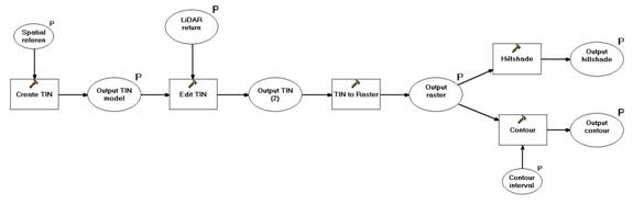
22. You are now ready to run the model. Close the ModelBuilder window. Exit out ArcCatalog and start ArcMap. In ArcToolbox, right-click ArcToolbox and select “Add Toolbox”. Browse to the folder where you saved the LiDAR Tools toolbox and add it to the ArcToolbox. In Arctoolbox, click the plus sign next to the LiDAR Tools toolbox, right click on the model you just created, and select Open (or just double-click it). Note that various parameters may not be in a logical order. Let’s fix that before we run the model.

23. Right-click on the model in ArcToolbox and select Edit.

24. Click on the ModelBuilder Model menu and select Model Properties. Select the Parameters tab. This is where you specify the order the parameters appear when you open the model. Put the parameters in the following order using the up/down arrows:

a. LiDAR return layer to process

b. Spatial reference of LiDAR returns

c. Output TIN model

d. Output raster elevation model

e. Output hillshade image

f. Contour interval (in feet)

g. Output contour shapefile

25. Save the model and close the ModelBuilder window. Open your model in ArcToolbox.

26. For the LiDAR return to process, select the first return point event layer you created in Task 1 (from the “LiDAR_Returns_First_Return _0503.dbf” table).

27. Press the button next to Spatial reference of LiDAR returns to specify a projection (for some reason, it cannot figure this out on its own from the projected returns.) Press the Import button, and browse to any of the datasets you created in Tasks 2 through 3 to copy the projection information from an existing dataset (or you can select the projection on your own).

28. Enter “5” as the Contour interval (in feet).

29. Input the parameters and name your outputs using the same protocols as you did in Tasks 2 through 3. Remember that you are processing the first return data this time, so name things accordingly (e.g., tin_fr, dsm_fr, etc.) (Note: Keep track of what you have changed and what you have not – ArcToolbox likes to fill in information for you even when it should not. Also note that you cannot overwrite datasets – they must be deleted first using ArcCatalog.)

30. Click OK to run the model. If you get an error, edit the model and fix any problems that it reports. See your instructor if you have problems you can’t resolve. Otherwise, you will see a dialog box reporting on the progress of the model run. This is complex data (more complex than the bare earth returns) – it will take several minutes to process. Be patient.

Questions

1. What is the main advantage of automating this process? Under what conditions would it not be worth the effort?

2. Add one more “process” to your model, such as exporting a slope raster image, save it, and run the model again. Export an Enhanced Metafile (.emf) of the model by selecting the Model menu, selecting Export – To Graphic, then name your output emf file. Insert the emf to your lab report and turn it in with your lab questions.

3. Visually compare the bare earth DEM and the first return DSM. Also compare the hillshades. What is the height of the “domed” structure just west of the storage tanks?

4. Compare the contours (the first return contours will take a long time to draw at the full extent – you might want to zoom in). Does it make sense to create contours for the first return data? Why or why not? How might these contours be used?

Task 5 – visualizing the data in 3D

Instructions

Thisl task is to visualize the data you have created so far in 3D. We will use ArcGIS’s ArcScene for this task. It’s not the best 3D visualization software, but it (usually) gets the job done.

1. Save your MXD and close ArcMap.

2. Open ArcScene (in the Windows Start menu under ArcGIS).

3. Add the bare-earth DEM created in Task 2.

4. Right-click on the layer, select Properties, then select the Base Heights tab. Click on the Obtain base heights from surface option, and select the DEM from the drop-down menu. This will render the DEM in 3D using the elevation values from the raster pixels.

5. Click Raster Resolution and enter 10 into Cellsize X and Cellsize Y. This is the resolution to which ArcScene will generalize the DEM (to make it draw faster). If you wanted the DEM to render at its full resolution, you would enter 5 for each value.

6. Click on the Rendering tab. Under Effects, check on Shade areal features relative to scene’s light position. Also, drag the Quality enhancement slider bar a bit to the right, so that the slider sits about 2/3 of the way to “high” (to improve the quality of the rendering).

7. Click the Symbology tab. Select a more colorful Color Ramp.

8. Click OK.

9. Repeat steps 1 through 8 with the first return DSM.

Questions

1. Note that the model has some irregularities on the southern edge. What are some possible ways to remove these kinds of edge issues when generating an elevation model?

2. Play around with the Raster Resolution layer property (in the Base Heights tab). Set it to the maximum resolution (5). For which model does it make the most difference visually? Why?

3. Where is this area?

Export a view of the full first return DSM from ArcScene (File – Export Scene – 2D). Print out a copy and turn it in with your lab.

Optional Task – creating a Terrain dataset in ArcGIS

Instructions

This task is for those who are interested in using the Terrain dataset in ArcGIS. Terrain dataset is a new data organization tool in ArcGIS for terrain data. It allows users to put all terrain related data such as, Lidar mass points, GPS points, breaklines, polygons, contours, etc, of a project in one place, i.e., a terrain dataset. A terrain dataset can only be created within a feature dataset. That means all the terrain data have to be in the same projection. Use Arccatalog to complete the following steps and examine the final product in ArcScene.

1. Create a file geodatabase (GDB) in your workspace.

2. Create a new feature dataset in the GDB, specify the Oregon HARN Stateplane that you used in Task 1 as the projection.

3. To reduce the process time for this optional task, you can use the Subset_Polygon shapefile to select (i.e., select by location) the LiDAR mass points from the bare earth and the first return XY data and export the data points to the feature dataset as featureclasses.

4. Import the Contour_55.shp to the feature dataset. This polyline featureclass will be used as a breakline layer. Use 3D Analyst to convert this featureclass into a 3D featureclass, so that the nodes and vertices of the polylines have elevation data (i.e., 55 feet).

5. You could convert the LiDAR mass point featureclasses you imported into 3D featureclasses, so that you can view them in 3D in ArcScene. This step is not required for the completion of this task.

6. Now you can use the Bare Earth points and the contour layer to create a Bare_Earth terrain dataset. Right-click the feature dataset and select New – Terrain. Type a name for the Terrain dataset and select the LiDAR Bare Earth and the contour layers to participate in the terrain. Type 5 as the average distance between points and click Next. In the next dialog, set the Height Source of the Bare Earth layer to Z_VALUE and set the SFType of the contour as soft line. Click Next, accept the default pyramid type and click Next. In the next dialog, click Add to add the first window size. Then click Next to review the setup. Use the back button to change the setting or click Finish to complete.

7. You can use the tools in the Terrain toolset in the 3D Analyst toolbox to modify the terrain dataset. Once the terrain is modified, use the Build Terrain tool to update the terrain.

8. Use “terrain” as the keyword to search Arctoolbox and see what tools are available for processing terrain datasets.