Lab 4. Change Detection and Change Vector Analysis

Introduction

We will use Landsat MSS images from two dates, 1985 and 1990, to map the areas where land-cover has changed over the period. The ERDAS IMAGINE function, “Modeler” will also be introduced in this lab. The lab data file (nalca.img) is in I:\Students\Instructors\Geoffrey_Duh\GEOG4582\Lab4. Please copy the file to your own folder before starting the exercise. Please answer all 3 questions. Submit the answers with the associated images to the instructor by the due date.

The data set that you will use is the North American Landscape Characterization (NALC). The NALC project is principally funded by the EPA Office of Research and Development's Global Warming Research Program and the USGS' Earth Resources Observation Systems (EROS) Data Center. The objectives of the NALC project are to develop standardized remotely sensed data sets and standard analysis methods in support of investigations of changes in land cover in North America related to land conversion (e.g. deforestation, agricultural expansion or abandonment, urbanization).

The NALC project includes Landsat MSS data acquired in the years 1973, 1986, and 1991, plus or minus one year, with geographic coverage including the conterminous United States and Mexico. The specific temporal windows vary for geographic regions based on the seasonal characteristics of the vegetation cover. The NALC “triplicate” scenes (one scene for each decade) are geographically referenced to a 60- by 60-meter UTM ground coordinate grid. Images from three dates are correctly co-registered with an individual RMS error smaller than 1.0 pixel.

We will use only a subset of the 80s (08/09/85) and 90s (08/31/90) NALC data WRS-2: Path 20, Row 31. The subset we will use covers the area of the City of Ann Arbor and vicinity. The following table summarizes the characteristics of MSS bands.

Band number	Band description	Bandwidth (mm)	IFOV (meter)
1	Green	0.5-0.6	79 – 82 (60*)
2	Red	0.6-0.7	79 – 82 (60)
3	Near infrared I	0.7-0.8	79 – 82 (60)
4	Near infrared II	0.8-1.1	79 – 82 (60)

* NALC data are resampled to 60- by 60-meter resolution.

There are many different change detection methods (see Jensen’s textbook). We will use the spectral change vector analysis method (CVA - see p.484) to process the 80s and 90s NALC data. Most change detection methods are sensitive to spectral differences between images that are not necessarily a result of land-cover change. Failure to understand the impact of various environmental characteristics on the remote sensing change detection process can lead to inaccurate results. The major non-land-use change environmental characteristic for the images we use is the variation of atmospheric and illumination conditions. Thus, an Automatic Scattergram-Controlled Regression (ASCR) radiometric rectification process (Elvidge et al. 1995) has already been done on your images from the 80s to match the atmospheric and illumination condition of the 90s (see Lab 3).

Exploring Change

We can visually explore the change first. Open nalcaa.img in a viewer, and set the band combination to Red: 4, Green: 8, Blue: 8. To facilitate this exercise, the following table summarizes the bands in the nalcaa.img file.

Band #	Layer name	Description
1	NALC_80_ch1	80s Green (MSS bnad1)
2	NALC_80_ch2	80s Red (MSS band2)
3	NALC_80_ch3	80s NIR I (MSS band3)
4	NALC_80_ch4	80s NIR II (MSS band4)
5	NALC_90_ch1	90s Green (MSS bnad1)
6	NALC_90_ch2	90s Red (MSS band2)
7	NALC_90_ch3	90s NIR I (MSS band3)
8	NALC_90_ch4	90s NIR II (MSS band4)

We set the 80s NIR II to red display channel and 90s NIR II to green and blue channels. If there were no changes between 80s and 90s images, then the image in the viewer would look in a gray tone. That’s how most areas within the interstate highway belt around the City of Ann Arbor look. (If you are not familiar with Ann Arbor and adjacent areas, please consult a google map to locate the city and highways.) When the 80s NIR II DN values are high and the 90s DN values are low, the pixels are shown in red tones. The pixels displayed in cyan tones show just the opposite.

Question 1: What could be the land-cover change scenario(s) for the red areas and the cyan areas? In addition, please describe the spatial-temporal distribution of these changed areas. Hint: You can open nalcaa.img in viewer #2 and #3 and set the band combinations of viewer #2 and viewer #3 to standard false-color infrared composites of 80s (3,2,1) and 90s (7,6,5) images respectively (see above table). You can geographically link all three viewers and use the “Inquire Cursor” interface to make the interpretation easier.

Change Vector Analysis

Next, we will actually map out these changed areas and the types of their change using the spectral change vector analysis. A spectral change vector describes land-cover change in terms of the change magnitude (CM) and direction of change from the earlier date to the later date. Change magnitude is computed by determining the Euclidean distance between the two images across all image channels on a pixel by pixel basis. Change direction is specified by whether the change is positive or negative in each band on a pixel by pixel basis. In this exercise, we will use all four MSS bands to calculate the CM and only use band 2 (red) and band 4 (NIR II) to specify the change directions. This means that we will examine only 4 instead of 16 change directions. The equation to calculate CM is:

where DN_ij is the digital number recorded in band j for date i.

The change directions in two-band spectral space are classified as follows:

	- Red +
- NIR II +	1	2
	3	4

where

If (DN₂₂-DN₁₂) < 0 and (DN₂₄-DN₁₄) < 0 then direction = 1

If (DN₂₂-DN₁₂) > 0 and (DN₂₄-DN₁₄) < 0 then direction = 2

If (DN₂₂-DN₁₂) < 0 and (DN₂₄-DN₁₄) > 0 then direction = 3

If (DN₂₂-DN₁₂) > 0 and (DN₂₄-DN₁₄) > 0 then direction = 4

A pixel in direction 3 shows an increase in Band 4 (NIR) and a decrease in Band 2 (Red). Therefore, this pixel is likely to be experiencing increase vegetation growth. A pixel in direction 2 shows a decrease in Band 4 and an increase in Band 2. Therefore this pixel has undergone a decrease in vegetation amount. A pixel that has increased both in Band 2 and 4 (i.e., in direction 4) indicates the land-cover of the pixel has changed to a high reflectance surface (e.g., parking lot).

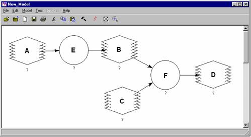
Change Magnitude and Modeler

Now, in the Imagine icon panel, click the “Modeler” icon, and then select “Model Maker”. After a blank model window and a tool panel appear, you will build your first model to calculate the CM image. Use the tool templates to duplicate the model in the diagram below to your blank model window. Click on the “Place a raster object” icon and the “Place a function” icon to select these object templates and click on the model window to add them to the model. Then click on the “Connect objects” icon and move the mouse pointer to the model window and place it within the object you just create. When the pointer turns into a downward arrow, click and drag the pointer into the target object. Repeat the steps to finish the model. When done, your model look like the one in the diagram.

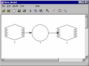
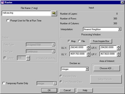
To define the object entities in the model, just double-click on the object. Double-click on the raster object to the left. A dialog appears. Select the nalcaa.img file as the associated raster layer and click OK. Repeat the same procedure for the raster object to the right and set the output file as fml_cm.img.

Next click on the function object to open the function definition dialog. You can just type in or select from (click on) the available inputs (buttons and list) to enter the following function into the blank field.

sqrt(($n1_nalcaa(5)-$n1_nalcaa(1))**2 + ($n1_nalcaa(6)-$n1_nalcaa(2))**2 + ($n1_nalcaa(7)-$n1_nalcaa(3))**2 + ($n1_nalcaa(8)-$n1_nalcaa(4))**2)

“$n1_nalcaa(5)” refers to the first object in the model and the fifth band in the input nalcaa.img file. “sqrt” stands for the square root function and “**” is the square operand.

Be sure to balance your parentheses!

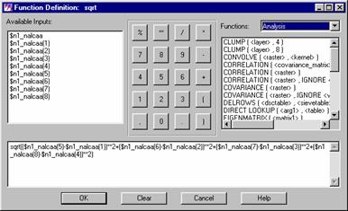
When done, click OK. The question marks in your model should now all disappeared. The model will process the nalcaa.img with the function specified and create an output raster file called fml_cm.img – all in your directory. To actually run the model, click on the “Execute the Model” icon . Now click on the icon to run the model. When done, save the model as fml_cmmodel. open the output raster file (fml_cm.img) in a new viewer and visually compare it to the image on viewer #1. The pattern in both images should look similar but not exactly the same. That is because the image on viewer #1 represents only the difference between one band while the CM image represents the aggregated difference from 4 bands.

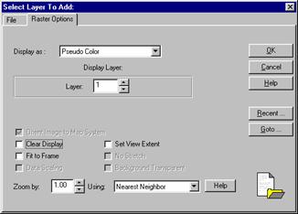
Now – very important step, you will select a threshold value above which change can be considered significant land-cover change, in comparison to changes that might result from the fluctuations of other environmental characteristics discussed in the textbook. The following procedures will make the selection of the threshold a little easier. Select the viewer in which you just opened the CM image and add the CM image to the viewer again - setting the following settings in the “Select Layer to Add” dialog. Set the “Display as” to “Pseudo Color” and disable the “Clear Display” checkbox, and then click OK.

The original CM image will be covered by a no-stretched darker CM image. Open the “raster attribute editor” dialog and set the “Opacity” of all records to 0 and the color to bright red. How to do this? First, to change all records at a time in a cell array, put the mouse pointer on the row header column, click right-mouse-button (RMB), and select “Select All”. Do this for the color column. Then click “Edit | Colors” on the viewer menu bar. Change slice method to: single color and start and end to red. All records will change to the same color. To change the numerical field, click on the column header cell (e.g., “Opacity”), click RMB and select all, and then click again and select “Formula”. Then enter the value or formula in the blank formula field (enter “0” in our case) and click “Apply”. Now, the bright CM image reappears on the viewer because the dark CM image (the active layer) became transparent (opacity = 0). You want to switch the opacity values on the transparent image back to 1 for records that have CM values larger than or equal to the threshold you will select (they will then show up in red). A good approach is to start with the highest CM values as they likely really are change and then begin changing the increasingly lower values one by one until you get to a threshold value that is questionable as to whether it is truly land-cover change or just a minor variation between the two images. By adjusting the opacity values for records around the tentative threshold value, you can visually assess the threshold for significant changes.

Question 2: Please report on your observations of the similarity and difference between the NIR II differencing image and the CM image. In your report also incorporate the screen-shot image of the colored changed areas, the histogram of the CM image, and the threshold value of the significant CM.

Change Direction and Modeler

Now, you should have a final value for the CM threshold. We will build another model to create the change direction map. Open a new model maker window, and follow the diagram below to create your model. Make sure you create A first, then B, C, D, E, and F. If you sequence is wrong, you will need to start from scratch.

Then, associate (all in your directory):

· A with fml_cm.img

· B with fml_chg.img

· C with nalcaa.img

· D with fml_chgdir.img

and set the functions of E and F to:

· For E:

CONDITIONAL { ($n1_fml_cm >= XX) 1 , ($n1_fml_cm < XX) 0 }

(Replace XX with your CM threshold value.)

· For F:

CONDITIONAL { ($n2_fml_chg == 1 and $n3_nalcaa(6) - $n3_nalcaa(2) < 0 and $n3_nalcaa(8) - $n3_nalcaa(4) < 0) 1 , ($n2_fml_chg == 1 and $n3_nalcaa(6) - $n3_nalcaa(2) > 0 and $n3_nalcaa(8) - $n3_nalcaa(4) < 0) 2 , ($n2_fml_chg == 1 and $n3_nalcaa(6) - $n3_nalcaa(2) < 0 and $n3_nalcaa(8) - $n3_nalcaa(4) > 0) 3, ($n2_fml_chg == 1 and $n3_nalcaa(6) - $n3_nalcaa(2) > 0 and $n3_nalcaa(8) - $n3_nalcaa(4) > 0) 4 }

Function E performs a thresholding and sets all changed areas in the output image (fml_chg.img) to 1, otherwise to 0. Function F specifies the rules to assign change direction codes (1 to 4) to the output image (fml_chgdir.img).

Note: The output files specified in the model shouldn’t already exist. So, if you execute the model and the model is interrupted by an error, make sure you first remove (delete) the intermediate output files that have been created.

When done, click the icon to execute the model. Then, open the nalcaa.img and display the 90s images with Red: 8, Green: 6, Blue: 5 combination if you haven’t done so. Use the “Pseudo Color” display type and disable “Clear Display” checkbox, and add the fml_chgdir.img to the viewer. Apply the skills you learned in previous lab sessions to make the viewer display the change areas clearly and meaningfully.

or

Open the fml_chgdir.img in one viewer, and the 80s and 90s false-color IR composites of the nalcaa.img in two other viewers and then link them all geographically.

You can color-code the fml_chgdir.img to correspond to the type of change (change direction). Open the Raster Attribute Editor and add a new column to the table called land-cover change. To add a new column, select Column Properties… from the Edit pulldown menu, set its type to “string”, then click on the New button. In this column color code the change direction and assign the labels a) increased veg, b)decreased veg, c) increased brightness, d) and decreased brightness. Refer to the explanation of change direction and associated table in this document to understand the information you are coding.

Question 3: Now you have a map (screen-captured copy of the viewer) of land-cover change of the City of Ann Arbor from 1985 to 1990. Please incorporate the map and the completed Raster Attribute table in your report and describe more specifically what types of land-cover change occurred. Do these land-cover changes indicate the way people use the land (i.e., land-use) has also changed?

Reference:

Elvidge D.C. et al. 1995. Relative radiometric normalization of Landsat multispectral scanner (MSS) data using an automatic scattergram-controlled regression. Photogrammetric Engineering & Remote Sensing, 61(10):1255-1260.