Lab 3: Relative radiometric normalization using automatic scattergram-controlled regression (ASCR)

Introduction:

In our next Lab (Lab 4), we will do a change vector analysis to identify land-cover change. Such a change detection method uses images that have the same radiometric characteristics. Most satellite images, due to atmospheric interference, require radiometric normalization to make a change vector analysis work. This exercise introduces an ASCR method (Elvidge et al 1995) for doing radiometric normalization. We use the images from 1972 and 1975 MSS to study the dynamics of vegetation near Mt. St. Helens in Washington.

ASCR method involves the delineation of no-change areas (NC) on the images based on NIR bands and uses the DN of the pixels in NC to calculate a regression model, then, applies the regression coefficients to normalize the DN of one image (i.e., subject) to the other (i.e., reference). We will use 1972's image as the subject and 1975's image as the reference.

Reference:

Elvidge, C.D. et al. 1995. Relative radiometric normalization of Landsat MSS data using an automatic scattergram-controlled regression. PE&RS 61(10):1255-1260.

The document is I:\Students\Instructors\Geoffrey_Duh\GEOG4582\Readings\Elvidge_etal_1995.pdf.

Instructions:

1. The lab data files (sthelens_mss.img and regression_imagery.gmd) are in I:\Students\Instructors\Geoffrey_Duh\GEOG4582\Lab3. Please copy the files to your own folder before starting the exercise. The model, regression_imagery.gmd, is also available at http://gis.leica-geosystems.com/Support/. Turn in this document with all the tables completed.

2. Open sthelens_mss.img in two viewers using the following band combinations of 4, 2, 1 (RGB) and 8, 6, 5 (RGB). Visually inspect the tone, color, and changes on both images and use the table below to record the image statistics reported in the ImageInfo window.

	1972 MSS				1975 MSS
	Min	Max	Mean	Stdv	Min	Max	Mean	Stdv
Green
Red
NIR 1
NIR 2

3. There are four bands in an MSS image: 1) Green, 2) Red, 3) NIR1, and 4) NIR2. Only NIR1 and 2 (bands 3 and 4) are used in delineating the no-change areas (NC). The band assignment in the image is: 1) Green (Subject date, i.e., 1972), 2) Red (Subject date), 3) NIR1 (Subject date), 4) NIR2 (Subject date), 5) Green (Reference date, i.e., 1975), 6) Red (Reference date), 7) NIR1 (Reference date), and 8) NIR2 (Reference date).

4. The identification of NC is based on scattergrams. Click on the "Classifier" icon on the main menu and select "Feature Space Image…". Set sthelens_mss.img as the input. Set the correct path and output root name (sthelens_mss). (Note that the default output path might be different from where the input file is). From the feature space layers panel, select sthelens_mss_3_7.fsp.img, then use the Shift key and select sthelens_mss_4_8.fsp.img. Click OK to create the scatter plots.

Note: The image from the reference date should be plotted on the y axis and the image from subject date (i.e., image to be corrected) should be plotted on the x axis for the following procedures to work correctly! If the bands of the reference image are put at the beginning of the image (i.e., having smaller band numbers), then you will need to click on the Reverse Axes to correct the setting. There is no need to make the correction in this exercise.

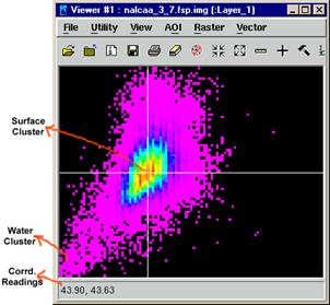
5.  Open both feature space images in viewers and identity the the local maximum coordinates of the water cluster (i_lmax,j_lmax) and the land-surface cluster (i_umax, j_umax) from both scatter plots of infrared channels (i.e., 3-7 and 4-8 feature space images). The picture below shows you how to determine the coordinates of these clusters.

6. Once you have the coordinates of these clusters, you then calculate a and b using the following equations:

Write down the values in the table below.

	iumax, jumax	ilmax,jlmax	a	b
Band 3-7 pair (NIR1)
Band 4-8 pair (NIR2)

7. a and b are used to estimate the half vertical width (HVW_NC) of no-change area from half perpendicular width (HPW_NC). We will use an HPW_NC value of 4 DN in this exercise. HVW_NC and HPW_NC have the following relationship:

You will calculate HVW_NC3 and HVW_NC4 for band 3 and 4 scatterplots using the “a” values of band 3 and 4. Based on experience, the values for HVW_NC shouldn’t be too large. The reasonable range is between 10 and 13 DN. Write down your HVW_NC3 and HVW_NC4 values below.

HVW_NC3

HVW_NC4

8. The mathematic definition of NC is:

 and

The as and bs in the equations are the a and b calculated in step 6. The ys are the DN of reference image (i.e., band 7 and 8) and xs are the DN of subject image (i.e., band 3 and 4). You need to create a model to delineate the NC. Follow the instructions at the end of this document (or on pages 379 to 390 on the ERDAS Imagine Tour Guide) to create a model that produces an image of the no-change areas. Use the EITHER…IF…OR…OTHERWISE function to assign the value indicating no-change areas in the output images. The logic, take NIR1 for example, is: if (band7 – b – a * band3) <= HVW_NC, then set the output pixel to 1, else, set output pixel to 0. The syntax is: EITHER 1 IF ((band7 – b – a * band3) <= HVW_NC3) OR 0 OTHERWISE. Note that you need to modify the statement to match the variable names of input files.

In the same spatial model, you can combine the no-change areas from both NIR bands with the “AND” function.

9. The next step is to create AOI from the image (i.e., NC mask) created in step 8. To create an AOI from a raster layer mask, the raster layer must be a pseudocolor layer (i.e, set “display as” to “pseudo color” in the raster option tab when you open the raster layer in the viewer). From the menu bar of the Viewer, select Raster | Attributes...The Raster Attribute Editor is opened. Then, select the class(es) you want to use to create the AOI. Here, you select the value (class) (i.e., 1) you assigned as no-change area in step 8. Select AOI | Copy Selection to AOI... If an AOI layer already exists, then the new area is added to it. If an AOI layer does not already exist, then it is created and the new area is added to it. Now, save the AOI to a new AOI file.

10. After the no-change areas have been identified, only pixel values within the no-change areas are used to estimate the regression equations for all pairs of bands from two dates. This needs to be done for green, red, NIR1, and NIR2. Open the modeler and load “regression_imagery.gmd” file. Set the input image file name and specify the AOI file you created in step 9 as the AOI. Set X-band to the bands from the subject image and Y-band to the bands from reference image. Set a and b to a.sca and b.sca. Execute the model, then read the values in the a.sca and b.sca files. Repeat the calculation for all bands and write down the as and bs.

Band	ak	bk
1
2
3
4

11. The coefficients (a_k and b_k) from these equations will be used to normalize the subject image (x_k). The normalized image () is derived with the equation:

You need to create models to finish the radiometric rectification process based on these regression equations for each band individually.

12. When done, use the Layer Stack tool in the Interpreter/Utilities menu to merge individual bands created in Step 11 and visually inspect the normalized and the reference images and use the table below to record the image statistics reported in the ImageInfo window.

	1972 MSS (normalized)
	Min	Max	Mean	Stdv
Green
Red
NIR 1
NIR 2

ERDAS Imagine Modeler

Click the “Modeler” icon in the Imagine icon panel, and then select “Model Maker”. After a blank model window and a tool panel appear, you will build your model to produce an image of the no-change areas. Use the tool templates to duplicate the model in the diagram below to your blank model window. Click on the “Place a raster object” icon and the “Place a function” icon  to select these object templates and click on the model window to add them to the model. Then click on the “Connect objects” icon and move the mouse pointer to the model window and place it within the object you just create. When the pointer turns into a downward arrow, click and drag the pointer into the target object. Repeat the steps to finish the model. When done, your model look like the one in the diagram.

To define the object entities in the model, just double-click on the object. Double-click on the raster object to the left. A dialog appears. Select the sthelens_mss.img file as the associated raster layer and click OK. Repeat the same procedure for the raster object to the right and set the output file as nc_mask.img.

Next click on the function object to open the function definition dialog. You can just type in or select from (click on) the available inputs (buttons and list) to enter the function into the blank field.

EITHER 1 IF ((abs($n1_sthelens_mss(7) – b₃ – a₃ * $n1_sthelens_mss(3)) <= HVW_NC3) AND (abs($n1_sthelens_mss(8) – b₄ – a₄ * $n1_sthelens_mss(4)) <= HVW_NC4)) OR 0 OTHERWISE

“$n1_sthelens_mss(7)” refers to the 7th band in the input sthelens_mss.img file. “abs” stands for the absolute function. Be sure to balance your parentheses!

When done, click OK. The question marks in your model should now all disappear. The model will process the sthelens_mss.img with the function specified and create an output raster file called nc_mask.img – all in your directory. To actually run the model, click on the “Execute the Model” icon . Now click on the icon to run the model.