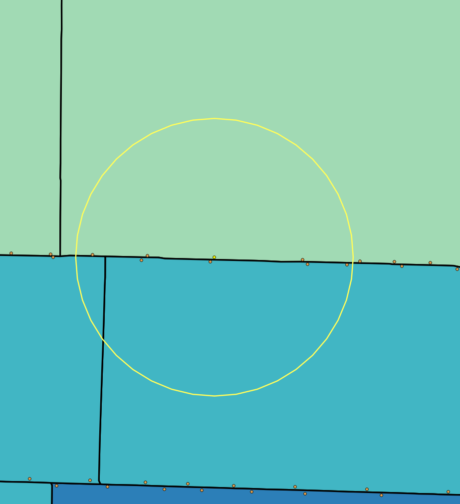
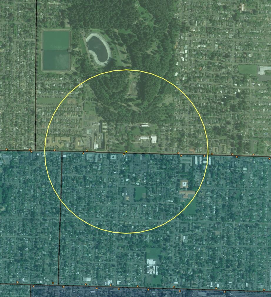
Figure 1. Proportional overlap method (left) includes part of uninhabited park (right)
Problem | Data | Method | Results | Discussion
Often, we encounter the problem that two interesting data sets don’t align. Or, the resolution of one data source is too coarse for our analysis question. Dasymetric mapping is a (pre-GIS) cartographic analysis method for improving density and distribution estimates by treating areas inside administrative boundaries as non-homogeneous. Put simply, it allows us to take an area total (e.g. census tract estimate) and use a secondary dataset with finer resolution to re-allocate the total within the larger area.
In this example, the specific problem was calculating poverty population at Census Tract level within transit stop buffers. A naive method that allocates proportionally based on overlap is compared with a dasymetric method using parcel-level land use data.
Figure 1. Proportional overlap method (left) includes part of uninhabited park (right)
We need two pieces of information for dasymetric mapping:
We'll use the ancillary data to better apportion poverty estimates within 1/3 mile airline buffers around frequent transit stops in Portland, Oregon.
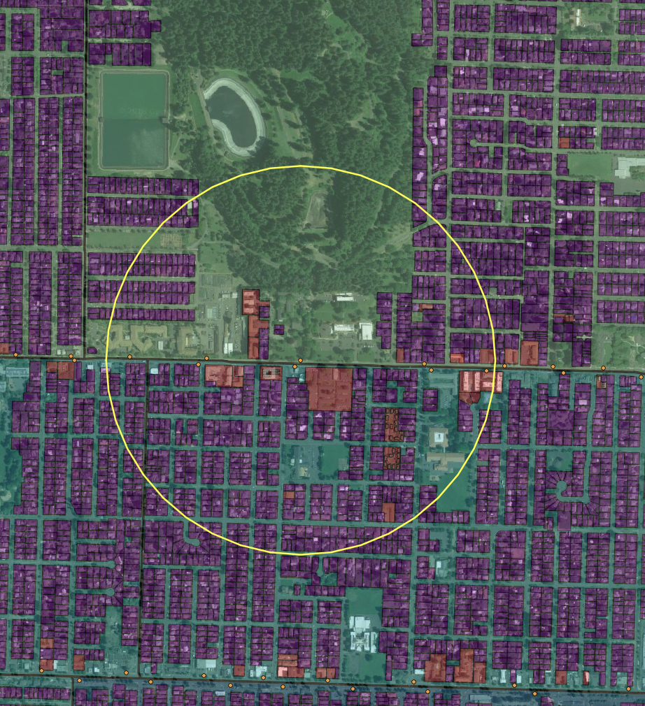
Figure 2. Three overlapping data sources (from bottom layer) census tract poverty estimates, taxlot land use, and transit stop buffers
Data were clipped to the city of Portland boundary.
The basic dasymetric method was as follows:
Attempts were made to complete the analysis in two desktop GIS environments (ArcMap & QGIS). However, it was difficult (QGIS) or impossible (ArcMap) to consistently produce the large vector spatial joins and intersects necessary for the dasymetric analysis. The PostGIS spatial database environment was chosen instead using the following procedures.
-- calc naive stop pop_pov as share area per tractWITH t1 AS (SELECT stops.LOC_ID, stops.RTE, stops.DIR, tracts.FIPS,(st_area(st_intersection(tracts.geom, stops.geom)) / (5280^2) /tracts.tract_sqmi) * tracts.pop_pov AS pop_pov1FROM tracts, stopsWHERE st_intersects(stops.geom, tracts.geom)),
The select statement defines the columns that will be returned by this (sub)query in the format table.column. So we’ll return LOC_ID, RTE, and DIR from the stops table FIPS from the tracts table.
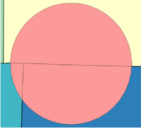
Figure 3. Naive (proportional area) slices per tract
-- sum residential bldg sqft per tractt2 AS (SELECT tracts.FIPS,sum(taxlots.BLDGSQFT):: double precision AS tract_sqftFROM tracts, taxlotsWHERE st_intersects(tracts.geom, taxlots.geom)group by tracts.FIPS),
Similar to the previous query, but the aggregation (dissolve) function in the select statement, sum(taxlots.BLDGSQFT), sums residential area by tracts.FIPS (the group by clause). This gives us total residential floor space per tract.
-- dasym calc pop_pov per taxlot per tractt3 AS (SELECT taxlots.rno,tracts.pop_pov * (taxlots.BLDGSQFT / t2.tract_sqft) AS lot_pop_povFROM taxlots, t2, tractsWHERE st_intersects(tracts.geom, taxlots.geom) ANDt2.FIPS = tracts.FIPS),
We can calculate the expected poverty population for each individual taxlot, since processing and memory constraints are no longer a big deal. We use our calculation from t2 to get each taxlot’s proportion of total tract area, and use that to apportion the total tract poverty population. We don’t bother slicing taxlots that straddle tracts; instead, they will appear in both tracts.
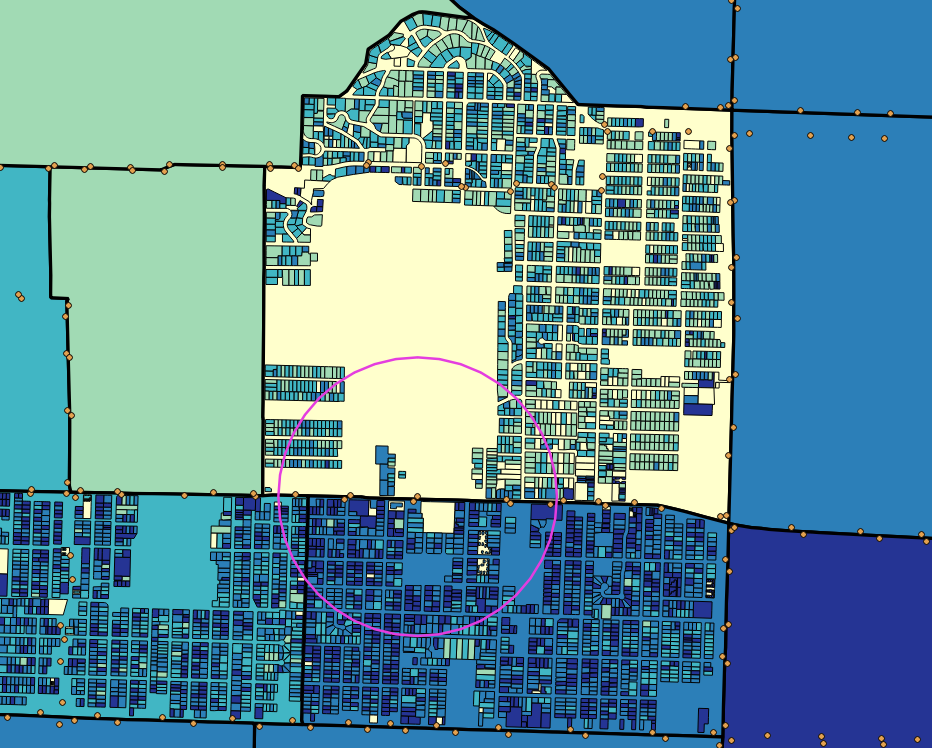
Figure 4. Estimated poverty density per taxlot, based on residential floor space and tract level total poverty population
t4 AS (SELECT stops.LOC_ID, stops.RTE, stops.DIR, sum(t3.lot_pop_pov) AS pop_pov2FROM stops, t3, taxlotsWHERE st_intersects(stops.geom, taxlots.geom) ANDt3.rno = taxlots.rnogroup by stops.LOC_ID, stops.RTE, stops.DIR),t5 AS (SELECT loc_id, rte, dir, sum(pop_pov1) pop_pov1FROM t1GROUP BY loc_id, rte, dir)
This is equivalent to a dissolve that sums taxlot level poverty population estimates from t3 by unique stop/route/direction combinations. In a Desktop GIS, you’d need to first create a single field that’s unique on stop/route/direction.
SELECT t4.loc_id, t4.rte, t4.dir, (t4.pop_pov2 - t5.pop_pov1)::integer AS pop_diff,t4.pop_pov2::integer, t5.pop_pov1::integerFROM t4 JOIN t5 ON (t4.loc_id=t5.loc_id AND t4.rte=t5.rte AND t4.dir=t5.dir)ORDER BY t4.loc_id, t4.rte, t4.dir;
Return the final output with only the columns we need. This could be joined to a stops layer (as in included dasym_out.sql to generate with geometry).
Results were examined by comparing the dasymetric estimates of poverty counts within transit buffers with those obtained with proportional area estimates. Differences were large in many cases (maximum differences over 1,000 people in poverty). The differences also appeared to be spatially correlated. For transit stops in the south end of downtown and along neighborhood arterials, the naive method seemed to under-predict poverty populations served, likely because dense residential development tends to be close to frequent transit service in those locations. In other areas of town near the river or in areas where transit stops near large commercial, industrial, or vacant (e.g. freeway area) land, a proportionally area method will likely overstate the residential population served by transit.
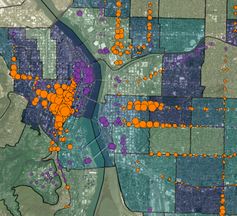
Figure 5. Results showing under- (orange) and over- (purple) estimates of poverty populations served within 1/3rd mile buffers when using naive, proportional area technique versus the dasymetric land use method
It is common in GIS planning analyses for data sources to align or overlap only partially. Decisions then have to be made about apportioning the different sources. In this exercise, two options were compared: 1) a common, relatively simple apportioning based on overlap of geographic area, and 2) a less common, more complex method that re-distributes a large-area aggregate based on related data with finer resolution. Both methods were applied to compare estimates of poverty populations falling within fixed distance buffers of public transit stops in Portland, Oregon
Results demonstrated that the choice of how to re-apportion aggregate data can have a large impact on results. Visual analysis also strongly suggested that the differences between methods were not randomly distributed across the study area.
A key disadvantage of the more complex (dasymetric) method is the need to establish additional assumptions about how the distribution of the original data correlates with an additional data source. For example, this analysis assumed those living in poverty were more concentrated in areas where residential floor space was higher, but that they were otherwise randomly distributed alongside other socioeconomic groups.
Another key limitation in the application context was the sole focus on residential access to transit. For simplicity, access to destinations was ignored.
A final limitation is the analysis and computational difficulty added by the dasymetric method. Using desktop GIS software was found to be unreliable, and the analysis was eventually completed using a spatial database system.
When assigning data across disjointed spatial areas, It's important to consider the impacts of different apportioning techniques. Large differences in results may occur across different methods. In cases where overlap between analysis and data areas are relatively small, it is worth exploring dasymetric techniques and ancillary data sources to potentially better represent the actual distribution of aggregated data. This should be balanced against the additional assumptions and complexity involved in applying techniques like the one shown here. Scripting and programmatic GIS environments such as spatial database packages can help with analysis reliability and computational constraints.