If you are reading this document as a web page, not a pdf, and prefer to read in Dark Mode, click the slider button in the top-right corner.

Prelude

The “for All” in the title of this document is meant to imply what it means: For people who write. We are discussing not just how to write computer code for data analysis with R and Python, we are also discussing how to write documents in general. Quarto document processing is revolutionary and accessible, as we will see.

To use quarto, within the RStudio environment on your computer instead of the cloud, you will need to download R and RStudio. You do not have to know much of anything about R to write documents with quarto. However, if you wish to learn about R for data analysis with RStudio, begin with these directions. If you are interested in Python and you need Python downloaded to your computer, try the Anaconda distribution.

If you have no interest in Python for data analysis, skip the next section and go straight to Quarto Markdown. There is no necessary reason to use Python or use R or use any data analysis system when writing documents with quarto. Sometimes we write documents to display and describe our computer output and sometimes we just write documents to say stuff.

Python in RStudio

See integrated for more details, but the basics are described below. Python integration in R is accomplish with the reticulate package, which provides the functions for interfacing Python with R and RStudio.

First, download the package from the R servers with the same procedure for any external, contributed R package.

install.packages("reticulate")

Once downloaded, retrieve the reticulate package from the R library with library(). Then, identify the location of the Python interpreter with the reticulate function use_python. The following example lists the default location of the anaconda download on a Mac.

library(reticulate)
use_python("~/anaconda3/bin")

If you are not an Anaconda Mac user, run the py_config() function to locate your Python language interpreter and replace the file reference in the use_python() function.

py_config()

When you know your Python location, you can save it indefinitely within RStudio.

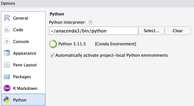
   Tools menu --> Global Options... --> Python

Enter the location. Then, there is no need to begin each Python session with the use_python() function.

Within RStudio, establish the location of Python for subsequent analyses.

Once the Python interpreter has been located, one possibility initiates an interactive Python session with the following function call:

repl_python()

The corresponding interactive prompt for a Python instruction is >>>. To have the Python instructions available for later use, store them in a file of Python code open in RStudio and copy lines of code into the interactive environment. See the next section for a more optimal strategy.

Quarto Markdown

Get Started

The modern way of writing, including creating documents that contain data analysis output, employs RStudio as a document preparation environment. This approach follows Donald Knuth’s concept of literate programming, in which a computer program becomes literature. This is the strategy used in creating this online reading. Use RStudio to write articles, books, slide shows, web sites, and blogs as text files formatted with markdown, specifically R Markdown, using the quarto document system. Create documents that not only contain static text but, if desired, analysis output from R or Python (and others) in text or slide format, directed to a web page, MS Word, or a pdf document.

Knuth, Donald E. 1984. Literate Programming. Comput. J. 27 (2): 97–111.

The term document in this context is ambiguous because there are two documents when working with markdown. The initial markdown document is a simple text file with embedded markdown codes. For example, in the in the markdown document if you want a word italicized, enclose the word within a beginning _ and ending _. Transform this text file by clicking the RStudio Render button into the corresponding rendered document used for presentation, which can be in various formats, such as a webpage or MS Word. Get a quick summary of R Markdown tags to embed in your document from the RStudio Help menu, Markdown Quick Reference.

To begin the preparation of any document, including one that contains R and/or Python code with included descriptive text, go to the Project drop-down menu at the far top-right of an RStudio window. Then, choose an Existing Directory or New Directory as needed.

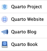
   Project drop-down menu --> New Project... --> New Directory --> Quarto Project

View a video of the document creation process from doing this menu sequence to creating the final document.

Choices offered for various types of `quarto` document formats.

To create the correct templates, choose Quarto Book format if multiple markdown documents (chapters) and a reference section are needed.

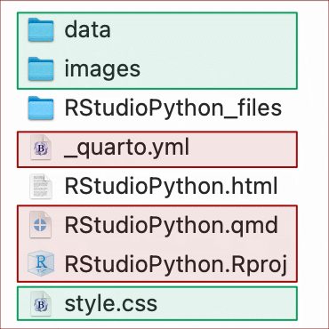
This RStudio menu sequence creates a directory for a minimal Quarto Project that renders a single document, complete with three files:

Markdown document, a text file with file type.qmdfor quarto markdown
RStudio project file with file type .Rproj, open this file to work on the document
YAML file named _quarto.yml for configuring aspects of document layout, which can be left unmodified for the default configuration

The directory structure for a quarto project for the document you are now reading, named RStudioPython, is illustrated below. The files listed in the folder are what occurred after the web output was rendered, the .html file, which is the primary output. Although not necessary, to help organize your files, add the following information to the project folder if relevant.

a data directory (folder) if one or more data files are referenced in the document
an images folder if .png images are to be embedded in the document
a .css file if you wish for custom styling of web output, though the default styling works well without the need for customization.

A `quarto` document directory (folder) for web output with the three files created by the `New Project` menu sequence highlighted in red and the optional folders/files manually created highlighted in green.

Use this ready-to-run basic .qmd sample document file created by RStudio as the basis for creating your markdown documents that can also run code. From this automatically created sample document, you can immediately begin revising and adapting to your own writing and analysis, either in Visual mode, similar to working with the usual word processor format, or in Source mode, where you can directly view and enter the markup instructions.

Push the Render button to generate a version of your document in the default web format, an .html file, or MS Word or a pdf output.

If needed, create a new .qmd document, within RStudio do File –> New File and then select either Quarto Document... for a standard document or Quarto Presentation... for a slide show.

As indicated, the YAML file, _quarto.yml, dictates much of the configuration of the input and output of the process of generating documents. The file does not need modification as you can immediately start working with it unmodified and to render quarto web pages, Word docs, and (with some additional software) pdf documents.

The YAML configuration instructions are typically distributed across the beginning of the .qmd document and the corresponding .yml configuration file. For example, the following three lines of YAML code appear at the top of the .qmd file from which this webpage was generated.

First three lines of the `.qmd` file from which this document is generated, the `YAML` instruction for titling the document.

These same three lines appear at the top of the sample .qmd document generated by RStudio when beginning a new project. Of course, the specific title here is different from the sample document.

By default, an .html file is generated when the Render button is pushed. To instead send the output to MS Word, add the YAML instruction format: docx line, such as at the beginning of your document.

First four YAML lines of a `.qmd` document file that directs subsequent output to an MS Word document.

Use a text editor to prepare your markdown document, such as RStudio’s built-in text editor or any other text editor. Text documents are free of any specific application and can be read and written by many applications. With this strategy, if desiring a MS Word document, MS Word is not used to write the document, only for outputting from your .qmd file when rendered. The MS Word document becomes output instead of the usual input. Of course, the MS Word output document can be edited directly, but if you want to make changes, best to revise your .qmd document and re-render the output.

Virtually all my writing is embedded within a markdown document, so I primarily use a specialized text cross-platform editor called VIM to write and edit text. I also use RStudio’s editor, set in VIM mode, often with the markdown document open in both apps. However, RStudio’s editor by itself works well. When beginning working with text documents there is no compelling need to learn other editors, if ever.

R and Python Code

If you wish to include R or Python code in your .qmd document, define the code in chunks. The sample text document from following the above instruction illustrates document creation and programming. Following is a Python example that generates output each time this document is re-generated after new editing and revision from within RStudio by clicking the Render button. The code reads an Excel data file into the data frame named d. The (37, 9) that follows the Python code is Python output, which indicates the number of rows, 37, and number of columns, 9, of that data frame.

import pandas as pd
d = pd.read_excel('data/employee.xlsx')
d.shape

(37, 9)

Within the .qmd document, the above code Python code chunk is written as follows.

A Python code chunk embedded in a `.qmd` document.

Define a chunk of Python code with the line ```{python} and follow the code chunk with the line ```. As you would imagine, replace the python with r to define a chunk of R code immersed within your document.

Rendering the markup document generates an output such as a web page, complete with text and data visualizations output generated when running your embedded R or Python (or others) code. You can also include your own images, such as in the default .png format. Below is an example of an R code chunk to include your image, stored in the created images folder.

An example R chunk for including an embedded image.

Setting echo to FALSE means that this code chunk will not appear in the output, so only the image appears. The out.width parameter is what it says, it sets the width of the output relative to the page. The fig.asp parameter sets the aspect of the figure, height relative to width. The fig.align parameter here is to center the image. The value of the fig.cap parameter is the figure caption.

Your document is now simultaneously a word processing document and a computer program. Welcome to the modern world of data analysis.

Writing and data analysis now simultaneously occur within the same document.

There are many available options, such as hiding the code from being displayed, depending on user preferences, and including pre-existing images as well as data visualizations as part of the computer output. Quarto was also recently made available from the Jupyter Notebook environment.

Appendix: Sample `YAML` File

As indicated, beginning a new quarto project from within RStudio automatically creates a default YAML document configuration file, _quarto.yml. This file works perfectly fine to configure your rendered document. At the same time, there are many, many customized configurations that can be specified with that file. Below is the YAML file that was used to generate this document, so revise with your name as author. Of course, if you do not have a .css file called style.css in the same project directory as your .qmd document, then eliminate the .css line. Or, just copy my style.css file that was used in the rendering of this document.

As previously indicated, any subset of these YAML statements can also appear in the YAML header at the beginning of the .qmd document. However, having most of the YAML instructions in a separate file facilitates sharing that file with other documents, leading to a consistent format across a variety of documents. The following instructions are for a single article. Creating multiple documents requires the book format, as outlined above.

format:
  html:
    css: style.css
    callout-icon: false
    date: now
    date-format: "MMM D, YYYY hh:mm a"
    toc: true
    toc-depth: 4
    link-external-newwindow: true

author: "David Gerbing"
title-block-banner: true
reference-location: margin

theme:
  light: cosmo 
  dark: slate

editor: visual