Note: The following material on the lessR function pivot() is based on the vignette on the same topic. To view this and other vignettes, each of which provides explanation and examples on a specific topic, enter into R: browseVignettes("lessR").
What is the mean salary across various departments in a company? What is the mean salary across departments for men and for women? Answer to these questions with aggregation.
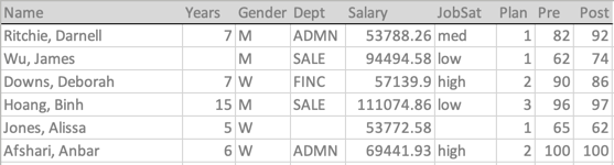
Listed below are the variable names and first six lines of the Employee data that serves as the example data illustrating aggregation.
Aggregating data results in a summary table, what Excel calls a pivot table. Choose a variable for which to compute a statistic over specified groups defined by the values of one or more categorical variables.
Consider the continuous variable Salary, for which a variety of statistics, such as the mean, may be aggregated. Different departments within the company define the groups, and then for each Gender within each department. One group is women in sales, another group is men in accounting, etc. For the statistic, choose the mean. To aggregate, compute the mean salary for each combination of the groups, the levels of Gender and Department.
Computing a pivot table with the lessR function pivot() or the Pandas function pivot_table() is the same process. The parameters that define these functions are imposed by the meaning of aggregation.
- data frame that contain the relevant variables
- statistic(s) to compute for the different groups
- (usually) numerical variable for which to compute the statistic
- categorical variables with the levels that define the groups
- optionally, choose to display the output as a data frame or a table
These five basic parameters of these two functions correspond to each of the above specifications, though with different names. The primary distinction is the mildly annoying Pandas requirement to enclose each variable name in quotes, here and for all functions.
In addition to the usual given statistics computations, such as the mean and the standard deviation, both pivot() and pivot_table() can aggregate the data with custom statistical functions. Any function applied to a variable, given or custom, must processes the data values for a single variable and return a single value for each group. However, pivot() does to some extent generalize beyond this limitation, providing output for three special functions discussed below.
R Aggregation
Prepare
To avoid clutter, suppress the usual output from loading these libraries and turn suggestions for alternative analyses off.
suppressMessages(library(lessR))
style(suggest=FALSE)
Read the Employee data.
#dR = Read('http://lessRstats.com/data/employee.xlsx', row_names=1, quiet=TRUE)
d <- Read('~/Documents/BookNew/data/Employee/employee.xlsx',
           row_names=1, quiet=TRUE)
Now verify the data that has been read.
dim(d)[1] 37 8head(d) Years Gender Dept Salary JobSat Plan Pre Post
Ritchie, Darnell 7 M ADMN 53788.26 med 1 82 92
Wu, James NA M SALE 94494.58 low 1 62 74
Downs, Deborah 7 W FINC 57139.90 high 2 90 86
Hoang, Binh 15 M SALE 111074.86 low 3 96 97
Jones, Alissa 5 W <NA> 53772.58 <NA> 1 65 62
Afshari, Anbar 6 W ADMN 69441.93 high 2 100 100Aggregate
To aggregate data, lessR provides the function pivot(), following the Excel name pivot table to describe the summary table of aggregated data.
Parameters
To use the pivot() function does not require complex computer code but a conceptual understanding of the process of aggregation. The parameter names are chosen so that describing an application is a regular English sentence.
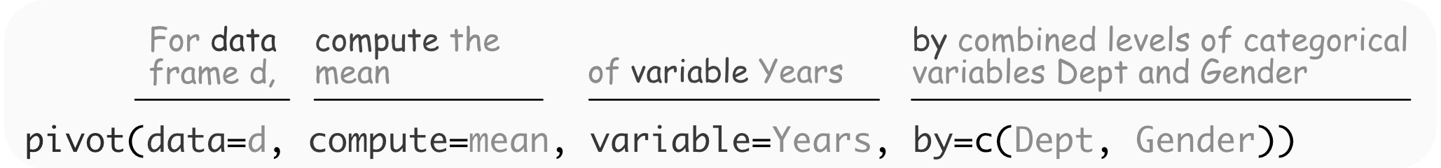
The first three listed parameter values are required to get one or more statistics computed over the entire data set. The fourth parameter, by, specifies the categorical variable(s) over which to aggregate, that is, compute the one or more specified statistics. If no by variables are specified, pivot() computes the specified statistics over all the data for the specified variables.
data: The data frame that includes the variables of interest.compute: The function(s) that compute the statistic(s) for which to perform the aggregation.variable: The variable(s) for which to summarize, i.e., aggregate.by: The categorical variable(s) that define the groups for which to compute the aggregated values.by_cols: The optional categorical variable(s) (not shown above) that define the groups for which to compute the aggregated values, listed as columns in a two-dimensional table for viewing instead of a data frame amenable for further analysis.
Multiple values of parameters variable, by, and up to two by_cols variables may be specified. Express multiple categorical variables over which to pivot as a vector, such as with the c() function. If by_cols is not specified, the result is a summary table as a long-form data frame that can be input into other data analysis procedures.
Missing Data
There are three different types of missing data in an aggregation: some missing values in a group for one or more aggregated variables for which the statistic is computed, all missing values for the variable in a group so that the group (cell) defined by one or more by variables has no data values, and the data value for the by variable itself is missing. Accordingly, there are three different missing data parameters with pivot().
na_remove: Remove any missing data from a value of thevariable, then perform the aggregation on the remaining values, reporting how many values are missing. Otherwise report the computed statistic as NA (missing) if even one data value is missing. [default isTRUE]na_by_show: If all values ofvariableare missing for a group so that the entire level of thebyvariables is missing, show those missing cells with a reported value of computed variable n as 0. Otherwise delete the row from the output. [default isTRUE]na_group_show: Thebydata value is missing so no data is available for any of the aggregated statistics, all displayed as missing values. Otherwise the row with the missingbydata value is deleted from the output. [default isTRUE]
To see examples of the application of these missing data parameters, refer to the section Missing Data in the pivot vignette at browseVignettes("lessR").
Statistical Functions
The following table lists many of the available R statistical functions by which to aggregate over the groups.
| Statistic | Meaning |
|---|---|
sum |
sum |
mean |
arithmetic mean |
median |
median |
min |
minimum |
max |
maximum |
sd |
standard deviation |
var |
variance |
IQR |
inter-quartile range |
mad |
mean absolute deviation |
tabulate |
count of each group only |
Some statistical functions are available that return multiple values.
| Statistic | Meaning |
|---|---|
range |
minimum, maximum |
quantile |
range + quartiles |
summary |
quantile + mean |
These later three functions output their values as an R matrix, which then replaces the values of the variable that is aggregated in the resulting output data frame. Custom functions can also be written for computing the statistic over which to aggregate.
To see how to define an R custom function, which can be accessed via pivot(), refer to the section Build Your Own Function in the pivot vignette at browseVignettes("lessR").
Output as a Data Frame
Two categorical variables in the d data frame are Dept and Salary. A continuous variable is Salary. Create the long-form pivot table as a data frame that expresses the mean of Salary for all combinations of Dept and Salary.
The first example is with no by variables. Simply compute the mean Salary for all of the Salary data values.
pivot(d, mean, Salary) n na mean
37 0 73795.56Now, add a by categorical variable to define the groups, here corresponding to each of the five levels of Dept. Compute the mean Salary for each Dept.
pivot(d, mean, Salary, by=Dept) Dept Salary_n na mean
1 ACCT 5 0 61792.78
2 ADMN 6 0 81277.12
3 FINC 4 0 69010.68
4 MKTG 6 0 70257.13
5 SALE 15 0 78830.07
6 <NA> 1 0 53772.58To aggregate over two categorical variables, create a vector of the two variables for the by parameter. This example includes the parameter names for emphasis, but if the parameters are entered in this order, their names are not necessary.
pivot(data=d, compute=mean, variable=Salary, by=c(Dept, Gender)) Dept Gender n na Salary_mean
1 ACCT M 2 0 59626.19
2 ADMN M 2 0 80963.35
3 FINC M 3 0 72967.60
4 MKTG M 1 0 99062.66
5 SALE M 10 0 86150.97
6 <NA> M 0 0 NA
7 ACCT W 3 0 63237.16
8 ADMN W 4 0 81434.00
9 FINC W 1 0 57139.90
10 MKTG W 5 0 64496.02
11 SALE W 5 0 64188.25
12 <NA> W 1 0 53772.58Or, as I usually write it, only including the name of the by parameter for readability.
pivot(d, mean, Salary, by=c(Dept, Gender)) Dept Gender n na Salary_mean
1 ACCT M 2 0 59626.19
2 ADMN M 2 0 80963.35
3 FINC M 3 0 72967.60
4 MKTG M 1 0 99062.66
5 SALE M 10 0 86150.97
6 <NA> M 0 0 NA
7 ACCT W 3 0 63237.16
8 ADMN W 4 0 81434.00
9 FINC W 1 0 57139.90
10 MKTG W 5 0 64496.02
11 SALE W 5 0 64188.25
12 <NA> W 1 0 53772.58The output of pivot() is a data frame of the aggregated variables. This summary table as a data frame can be saved for further analysis. Here, perform the same analysis, but save the result into the data frame a and the display the contents of a. Because the output of pivot() with no by_cols variables is a standard R data frame, typical operations such as sorting can be applied, here using the lessR function sort_by().
a <- pivot(d, mean, Salary, by=c(Dept, Gender))
sort_by(a, by=Salary_mean, direction="-")
Sort Specification
  Salary_mean -->  descending
Dept Gender n na Salary_mean
4 MKTG M 1 0 99062.66
5 SALE M 10 0 86150.97
8 ADMN W 4 0 81434.00
2 ADMN M 2 0 80963.35
3 FINC M 3 0 72967.60
10 MKTG W 5 0 64496.02
11 SALE W 5 0 64188.25
7 ACCT W 3 0 63237.16
1 ACCT M 2 0 59626.19
9 FINC W 1 0 57139.90
12 <NA> W 1 0 53772.58
6 <NA> M 0 0 NAOr, use the pipe operator to follow the linear flow from the original data d to summary data frame a. When piping data output from one function to the next, if the data for the receiving function is specified in the first parameter, then drop that parameter from the function call. Accordingly, the calls to pivot() and sort_by() have no specified data frame, otherwise listed as the first parameter for each.
d |>
  pivot(mean, Salary, by=c(Dept, Gender)) |>
  sort_by(by=Salary_mean, direction="-") ->
a
Sort Specification
  Salary_mean -->  descending
Multiple variables for which to aggregate over can also be specified. Here, round the numerical aggregated results to two decimal digits with the digits_d parameter.
pivot(d, mean, c(Years, Salary), c(Dept, Gender), digits_d=2) Dept Gender Years_n Years_na Years_mean Salary_n Salary_na Salary_mean
1 ACCT M 2 0 7.00 2 0 59626.20
2 ADMN M 2 0 15.50 2 0 80963.34
3 FINC M 3 0 11.33 3 0 72967.60
4 MKTG M 1 0 18.00 1 0 99062.66
5 SALE M 9 1 12.33 10 0 86150.97
6 <NA> M 0 0 NA 0 0 NA
7 ACCT W 3 0 4.67 3 0 63237.16
8 ADMN W 4 0 7.50 4 0 81434.00
9 FINC W 1 0 7.00 1 0 57139.90
10 MKTG W 5 0 8.20 5 0 64496.02
11 SALE W 5 0 6.60 5 0 64188.25
12 <NA> W 1 0 5.00 1 0 53772.58Output as a 2-D Table
Specify up to two by_cols categorical variables to create a two-dimensional table with the specified columns. Specifying one or two categorical variables as by_cols variables moves them from their default position in the rows to the columns.
Moving rows to columns changes the output structure from a long-form data frame that can be input into other analysis functions to a cross-classification table with categorical variables in the rows and columns. The primary purpose of the cross-classification table is to view the aggregated results, not to subject them to further analysis. For viewing, the tabular presentation can be easier to interpret.
In this example, the fifth value entered in the function call is the value of by_cols, Gender in this example.
pivot(d, mean, Salary, by=Dept, by_cols=Gender)Table: mean of Salary
Gender M W
Dept
------- --------- ---------
ACCT 59626.19 63237.16
ADMN 80963.35 81434.00
FINC 72967.60 57139.90
MKTG 99062.66 64496.02
SALE 86150.97 64188.25
NA NA 53772.58Here are two by_cols variables, specified as a vector.
pivot(d, mean, Salary, by=Dept, by_cols=c(Gender, Plan))Table: mean of Salary
Gender M W
Plan 1 2 3 1 2 3
Dept
------- --------- ---------- --------- --------- --------- ---------
ACCT 69547.60 NA 49704.79 NA 63237.16 NA
ADMN 53788.26 108138.43 NA NA 67724.21 122563.4
FINC 61937.62 NA 95027.55 NA 57139.90 NA
MKTG NA NA 99062.66 56772.95 66426.79 NA
SALE 89393.40 82442.74 80131.91 60941.54 66352.73 NA
NA NA NA NA 53772.58 NA NAThere are many NAs in the pivot table because there are only 37 rows of data that are divided into many groups, all combinations of the variables Dept (5), Gender (2), and Plan (3), so 30 groups total.
Tabulation
Tabulation is counting. The number of data values in each group are tabulated, that is, counted, their frequency of occurrence obtained. For the function that specifies what to compute, specify table.
pivot(d, table, Dept, by=Gender) Gender Dept_n na ACCT ADMN FINC MKTG SALE
1 M 18 0 2 2 3 1 10
2 W 18 1 3 4 1 5 5Note you can get the same joint frequency table from the lessR function BarChart().
BarChart(Dept, by=Gender)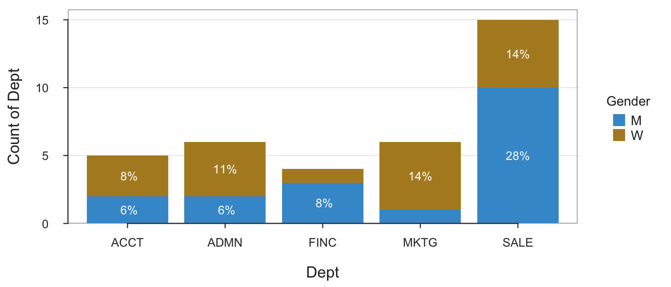
Joint and Marginal Frequencies
------------------------------

       Dept
Gender   ACCT ADMN FINC MKTG SALE Sum
  M         2    2    3    1   10  18
  W         3    4    1    5    5  18
  Sum       5    6    4    6   15  36

Cramer's V: 0.415

Chi-square Test of Independence:
     Chisq = 6.200, df = 4, p-value = 0.185
>>> Low cell expected frequencies, chi-squared approximation may not be accurate
Of course, many other functions are available from which to obtain the joint frequencies of the two categorical variables.
Base R Aggregation
The Base R function, upon which pivot() relies, is aggregate(). Express this function in one of two modes. This example is of formula mode.
aggregate(Salary ~ Dept + Gender, data=d, FUN=mean) Dept Gender Salary
1 ACCT M 59626.20
2 ADMN M 80963.35
3 FINC M 72967.60
4 MKTG M 99062.66
5 SALE M 86150.97
6 ACCT W 63237.16
7 ADMN W 81434.00
8 FINC W 57139.90
9 MKTG W 64496.02
10 SALE W 64188.25The aggregate() function is not as flexible nor as powerful as lessR pivot(), which takes the output of aggregate() and then offers the following enhancements.
- For each
valueover which to aggregate, the sample size and number of missing values for each group is provided. - Multiple statistical functions can be selected for which to
computethe aggregated value for each group. - Extends beyond aggregation to
computestatistics over the entire data set instead of groups of data. - Missing data analysis by group or by the
valueaggregated. - Aggregation not necessary, so can
computethe specified statistic(s) for eachvariableacross the entire data set. - The aggregated computations can be displayed as a 2-D table, not just a long-form data frame.
byvariables of typeDateretain the same variable type in the summary table instead of each converted to afactor(setfactors=FALSEto not convertintegerandcharactervariables to factors).- The list of parameters lists the
dataparameter first, which facilitates the use of the pipe operator, such as from base R as of Version 4.1.0 or the magrittr package. - Any non-numeric variables with unique values in the submitted
dataare listed with their corresponding data value, which identifies when drilling down into the data to study relevant rows.
Python Aggregation
Prepare
Import the needed modules.
import pandas as pd
import numpy as np
import seaborn as sns
Read the Employee data.
#df = pd.read_excel('http://lessRstats.com/data/employee.xlsx', index_col=0)
df = pd.read_excel('~/Documents/BookNew/data/Employee/employee.xlsx',
                   index_col=0)
Verify what was read.
df.shape(37, 8)df.head() Years Gender Dept Salary JobSat Plan Pre Post
Name
Ritchie, Darnell 7.0 M ADMN 53788.26 med 1 82 92
Wu, James NaN M SALE 94494.58 low 1 62 74
Downs, Deborah 7.0 W FINC 57139.90 high 2 90 86
Hoang, Binh 15.0 M SALE 111074.86 low 3 96 97
Jones, Alissa 5.0 W NaN 53772.58 NaN 1 65 62The following Pandas function provides much information regarding the data frame.
def details(df, brief=True):

    ty = df.dtypes
    nv = df.count()
    nm = df.isna().sum()
    nu = df.nunique()
    dStats = pd.concat([ty,nv,nm,nu], axis='columns',
                       keys=['type', 'values', 'missing', 'unique'])
    print(dStats)

    if not brief:
      print("\n")
      print(df[df.isna().any(axis='columns')])
Call this details() function with the current data frame, df.
details(df) type values missing unique
Years float64 36 1 16
Gender object 37 0 2
Dept object 36 1 5
Salary float64 37 0 37
JobSat object 35 2 3
Plan int64 37 0 3
Pre int64 37 0 27
Post int64 37 0 22From this information, we can identify that the following variables are categorical: Gender, Dept, JobSat, and Plan.
Aggregate
A primary Pandas function for computing and formatting a pivot table is pivot_table(), illustrated below.
Parameters
The first three listed parameter values of pivot_table() are required to get one or more statistics computed over the entire data set. The fourth parameter, by, specifies the categorical variable(s) over which to aggregate, that is, compute the one or more specified statistics.
data: The data frame that includes the variables of interest.aggfunc: The function(s) for the statistic(s) for which to perform the aggregation.values: The variable(s) for which to summarize, i.e., aggregate.index: The categorical variable(s) that define the groups for which to compute the aggregated values.columns: The optional categorical variable(s) (not shown above) that define the groups for which to compute the aggregated values, listed as columns in a two-dimensional table for viewing.
Statistical Functions
The following table lists many of the available R statistical functions by which to aggregate over the groups.
| Statistic | Meaning |
|---|---|
sum |
sum |
mean |
arithmetic mean |
median |
median |
min |
minimum |
max |
maximum |
std |
standard deviation |
var |
variance |
count |
count of each group only |
first |
first item in the data |
last |
last item in the data |
Output as a Data Frame
Unlike the lessR function pivot(), the following instance of using pivot_table() to compute the mean of Salary for all data values of Salary does not work. Groups must be specified, so a different function is required to compute the statistic over all the values of the variable, here Salary.
#pd.pivot_table(data=df, aggfunc='mean', values='Salary')Pivot on the categorical values of one categorical variable, Dept, indicated by the index parameter.
pd.pivot_table(data=df, aggfunc='mean', values='Salary', index='Dept') Salary
Dept
ACCT 61792.776000
ADMN 81277.116667
FINC 69010.675000
MKTG 70257.128333
SALE 78830.064667To aggregate over two categorical variables, create a vector defined as a Python list of the two variables passed to the index parameter.
pd.pivot_table(data=df, aggfunc='mean', values='Salary',
                        index=['Dept', 'Gender'])
Salary
Dept Gender
ACCT M 59626.195000
W 63237.163333
ADMN M 80963.345000
W 81434.002500
FINC M 72967.600000
W 57139.900000
MKTG M 99062.660000
W 64496.022000
SALE M 86150.970000
W 64188.254000The output of pivot_table() for groups defined by the combination of levels of two categorical variables is not a fully formed data frame. Presumably, to enhance readability, there are missing values for the first column of the output data frame. If the output summary table is to be further analyzed, it should be converted to a proper data frame. To do so, invoke the reset_index() function. Here, also save the output into the a data frame to be available for further processing.
a = pd.pivot_table(data=df, aggfunc='mean', values='Salary',
                            index=['Dept', 'Gender'])
a = a.reset_index()
a
Dept Gender Salary
0 ACCT M 59626.195000
1 ACCT W 63237.163333
2 ADMN M 80963.345000
3 ADMN W 81434.002500
4 FINC M 72967.600000
5 FINC W 57139.900000
6 MKTG M 99062.660000
7 MKTG W 64496.022000
8 SALE M 86150.970000
9 SALE W 64188.254000Here, sort the values of the pivot table as a proper data frame in descending order of Salary. Also, round the data values to two decimal digits with the round() function, added on to the function call to form a single statement.
a.sort_values(by='Salary', ascending=False).round(2) Dept Gender Salary
6 MKTG M 99062.66
8 SALE M 86150.97
3 ADMN W 81434.00
2 ADMN M 80963.34
4 FINC M 72967.60
7 MKTG W 64496.02
9 SALE W 64188.25
1 ACCT W 63237.16
0 ACCT M 59626.20
5 FINC W 57139.90Or, more elegantly, combine these operations into one statement.
a = (df
  .pivot_table(aggfunc='mean', values='Salary', index=['Dept', 'Gender'])
  .reset_index()
  .sort_values(['Salary'], ascending=False).round(2)
)
a
Dept Gender Salary
6 MKTG M 99062.66
8 SALE M 86150.97
3 ADMN W 81434.00
2 ADMN M 80963.34
4 FINC M 72967.60
7 MKTG W 64496.02
9 SALE W 64188.25
1 ACCT W 63237.16
0 ACCT M 59626.20
5 FINC W 57139.90As usual, there are multiple ways to accomplish the same goal. An alternative to pivot_table(), shown here because it also is frequently used, is based on the group_by() function. Here, the reset_index() function and round() are both included to form a single statement.
df.groupby(['Dept', 'Gender'])['Salary'].mean().reset_index().round(2) Dept Gender Salary
0 ACCT M 59626.20
1 ACCT W 63237.16
2 ADMN M 80963.34
3 ADMN W 81434.00
4 FINC M 72967.60
5 FINC W 57139.90
6 MKTG M 99062.66
7 MKTG W 64496.02
8 SALE M 86150.97
9 SALE W 64188.25Multiple variables for which to aggregate over can also be specified. Here, round the numerical aggregated results to two decimal digits with round().
pd.pivot_table(data=df, aggfunc='mean', values=['Years', 'Salary'],
                                        index=['Dept', 'Gender']).round(2)
Salary Years
Dept Gender
ACCT M 59626.20 7.00
W 63237.16 4.67
ADMN M 80963.34 15.50
W 81434.00 7.50
FINC M 72967.60 11.33
W 57139.90 7.00
MKTG M 99062.66 18.00
W 64496.02 8.20
SALE M 86150.97 12.33
W 64188.25 6.60Output as a 2-D Table
Moving rows to columns changes the output structure from a long-form data frame that can be input into other analysis functions to a cross-classification table with categorical variables in the rows and columns. The primary purpose of the cross-classification table is to view the aggregated results, not to subject them to further analysis. For viewing, the tabular presentation can be easier to interpret.
The fifth value entered into the following function call is the value of columns, Gender in this example.
pd.pivot_table(data=df, aggfunc='mean', values='Salary', index='Dept',
                        columns='Gender')
Gender M W
Dept
ACCT 59626.195 63237.163333
ADMN 80963.345 81434.002500
FINC 72967.600 57139.900000
MKTG 99062.660 64496.022000
SALE 86150.970 64188.254000Now, specify two columns categorical variables.
pd.pivot_table(data=df, aggfunc='mean', values='Salary', index='Dept',
               columns=['Gender', 'Plan'])
Gender M W
Plan 1 2 3 1 2 3
Dept
ACCT 69547.600 NaN 49704.79 NaN 63237.163333 NaN
ADMN 53788.260 108138.43 NaN NaN 67724.210000 122563.38
FINC 61937.625 NaN 95027.55 NaN 57139.900000 NaN
MKTG NaN NaN 99062.66 56772.95 66426.790000 NaN
SALE 89393.400 82442.74 80131.91 60941.54 66352.730000 NaNThere are many NaNs in the pivot table because there are only 37 rows of data that are divided into many groups, all combinations of the variables Dept (5), Gender (2), and Plan (3), so 30 groups total.
Set the margins parameter to True to add the row and column margins to the output. For example, the marginal means are the means of all the data across within each row or column.
pd.pivot_table(data=df, aggfunc='mean', values='Salary', index='Dept',
               columns=['Gender', 'Plan'], margins=True).round(2)
Gender M W All
Plan 1 2 3 1 2 3
Dept
ACCT 69547.60 NaN 49704.79 NaN 63237.16 NaN 61792.78
ADMN 53788.26 108138.43 NaN NaN 67724.21 122563.38 81277.12
FINC 61937.62 NaN 95027.55 NaN 57139.90 NaN 69010.68
MKTG NaN NaN 99062.66 56772.95 66426.79 NaN 70257.13
SALE 89393.40 82442.74 80131.91 60941.54 66352.73 NaN 78830.06
All 78357.15 91007.97 80811.76 59552.01 65342.10 122563.38 74351.75The default name of each margin is All. Customize the name with the margins_name parameter.
Tabulation
Here, tabulate the values in each group by specifying the aggregation function with parameter aggfunc as count. Order the counts into a table with the columns parameter.
pd.pivot_table(data=df, aggfunc='count', index='Gender', columns='Dept') JobSat Plan ... Salary Years
Dept ACCT ADMN FINC MKTG SALE ACCT ADMN ... MKTG SALE ACCT ADMN FINC MKTG SALE
Gender ...
M 2 2 3 1 10 2 2 ... 1 10 2 2 3 1 9
W 2 4 1 5 5 3 4 ... 5 5 3 4 1 5 5
[2 rows x 30 columns]