To create the interactive maps shown here requires the contributed R packages: tidygeocoder, sf, maps, and mapview. As always, these packages must be installed once, such as with the RStudio Tools menu, and then accessed with the library() function for each R session. Or, just run the following function call to install.
install.packages(c("tidygeocoder", "sf", "mapview", "maps"))Now access the packages from your R library with the following library() calls. With lessR, turn off the suggestions to save space and focus on the primary content.
suppressPackageStartupMessages(library(lessR))
style(suggest=FALSE)
library(tidygeocoder)
library(mapview)
library(maps)
library(sf)
Linking to GEOS 3.11.0, GDAL 3.5.3, PROJ 9.1.0; sf_use_s2() is TRUEMaps
From lessR version 4.4.1.
From mapview version 2.11.2.
From maps version 3.4.2.1.
From sf version 1.0.19.
Projections
The Earth is approximately spherical. We draw maps of the Earth on flat surfaces such as paper or a computer screen. To create a map we must transfrom spherical coordinates, which describe specific locations on a curved surface with three dimensions, into the two-dimensional x,y coordinates of a flat surface.
Flatten the coordinates of latitude and longitude that describe a position on the Earth’s three-dimensional surface into two dimensions.
All maps of any part of the Earth are projections. Unfortunately, a flat surface cannot represent a spherical object without distortion. There are many available competing projections, each with their own particular set of flaws. A transformation to flatness cannot simultaneously retain all of the following: accuracy of area, direction, distance, and shape. Each possible projection compromises at least one of these properties, focusing on minimizing the distortion in the others. The larger the area mapped, the more distortion encountered. A world map necessarily presents more distortion than a city map.
With modern computer technology, you can view a variety of projections or even create your own.
Figure 1 illustrates two different projections of the earth-s surface.
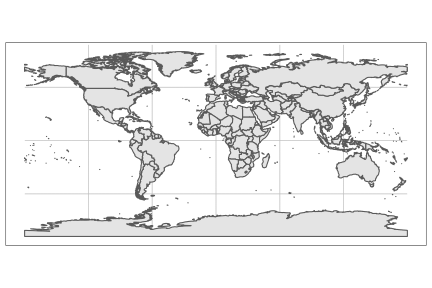
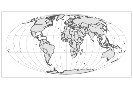
Figure 1 (a) presents one of the most straightforward, simpler projections, the rectangular projection, which linearly plots latitude and longitude directly into coordinates in the x-y plane. This projection renders the Earth as a flat rectangle, necessarily resulting in much distortion. For example, the Antarctic is not many times larger than North America.
The Mollweide projection in Figure 1 (b) renders a more sophisticated map of the Earth with much less distortion of the sizes of the continents. However, there is some loss of accuracy of angles between the continents and their shapes. The Mollweide projection follows from a non-linear transformation of the spherical coordinates of latitude and longitude into the coordinates of the map’s x-y plane.
Map Types
There are many types of maps. The following are among the most common types.
- Political map or country map: shows political and administrative boundaries, such as countries and states within countries, and cities within states, what Tableau calls a symbol map when plotted symbols represent geographical entities such as cities and possible the size of the plotted symbol reflects the extent of the value of some variable such as population. With a small enough area that shows streets and highways, this map can be called a street map.
- Choropleth map or thematic map: fill in different parts of the map with varying intensities of color, what Tableau calls a filled map, where the color intensity reflects the value of some other variable
- Physical map or terrain map: shows natural landscape features of the Earth, what Tableau calls a satellite map when created from imagary of the world
We will use the mapview() function from the package of the same name to create maps in these three styles.
Visualization Modes
Store a digital image in one of two primary formats: vector or raster.
Composed of paths defined by mathematical formulas, including points, lines, and curves.
Vector images are resolution independent, so they scale perfectly from small to large with no distortion because they consist of mathematical descriptions of objects. Viewing a vector image is viewing the display of mathematical objects created at the given resolution. They are informally referred to as drawings, roughly analogous to a human-created drawing with pen and paper that has the advantage of scalability. Common file types are .pdf and .eps.
Vector images can scale perfectly, but without the finest level of detail and gradation that a photograph can provide, which represents the other primary type of image.
Composed of a grid of pixels, each having a specific color value.
A photograph is a raster image, typically composed of a large number of tiny pixels or dots. The disadvantages are that raster images can require much storage space compared to vector images and distort when scaled to larger images. A raster image, however, at its native resolution, can achieve precise detail, detailed textures with a gradation of colors. A raster image is also called a bit-mapped image or more informally, a painting or photograph. Common file types are .jpeg or .jpg, and .png.
Figure 2 presents an example of each type of image.


The key for map making is that historically raster images were required to construct detailed maps. Now, quality maps also can be constructed from vector images. Raster maps can also be constructed from visualization systems but given the successful development of the more flexible vector images, that is all that will be covered here.
Geocodes
Access the Geocodes
If we wish to plot geographical objects such as cities on a map, to identify each object we need its location.
An object’s location in terms of longitude and latitude.
Obtain geocodes from location-based data, such as such as street addresses or place names. We have two ways to obtain these geocodes. One method uses an online service for the specific addresses of places we provide, and the other accesses data files on the web that include geocodes for existing geographical features, such as cities around the world. Of course, the advantage of custom geocodes is that we can customize the resulting map to the specific locations of interest.
Once the geocodes are obtained for the desired locations, creating the resulting map is straightforward.
Custom Geocodes
Visualization systems typically provide multiple methods to obtain custom geocodes. For R, we will use the geocode() function from the tidygeocoder package to obtain the geocodes. You can present the address for each object as a single character string or divide it into separate variables that specify the street, city, state, and ZIP Code.
One advantage of using this geocode() function is that the data file you submit to the function can contain additional information that will remain part of the resulting geocoded file.
In addition to locations, your geocode data file can contain other information useful to visualize such as number of employees for company locations, and financial data such as revenue, sales, and profitability.
Each of these different variables can be visualized on a map such as creating a bubble plot where the size of the plotted point represents the intensity of the corresponding variable.
Figure 3 shows the information contained in an Excel file that will be input into the geocodes() function. The variables can have any name. The only variable needed to get the geocodes is the address of each location. Suppose we are a business that sells some service or product to the following locations.
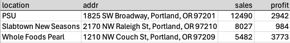
Prepare to obtain the geocodes by first reading the address file into R, such as into the g data frame.
g <- Read("data/addresses.xlsx", quiet=TRUE)The call to geocode() is straightforward. The first parameter is the data frame of the addresses, followed by the address parameter that references your column of addresses from the Excel worksheet. Several online services provide the geocodes from which geocodes() will obtain that information. The geocoding service used here is Open Street Maps, specified by the method parameter as "osm".
g <- geocode(g, address=addr, method="osm")Passing 3 addresses to the Nominatim single address geocoderQuery completed in: 3.3 secondsg# A tibble: 3 × 6
location addr sales profit lat long
<chr> <chr> <int> <int> <dbl> <dbl>
1 PSU 1825 SW Broadway, Portland, OR 97201 12490 2942 45.5 -123.
2 Slabtown New Seasons 2170 NW Raleigh St, Portland, OR 97210 8027 984 45.5 -123.
3 Whole Foods Pearl 1210 NW Couch St, Portland, OR 97209 5482 3773 45.5 -123.The only annoying aspect of the geocode() function is that it does not return a standard R data frame. Without getting too sidetracked here, the RStudio people are trying to take over R by introducing a different dialect of R that works the same without any clear advantages in general. Their often effective propaganda that their dialect is superior is simply not true in general. They do not even use standard R data frames but instead use something called a tibble, similar but different. To convert the output tibble to a standard R data frame, add the code g <- data.frame(g). However, this conversion is not necessary as the downstream functions must also process tibbles for compatibility, just as do my lessR functions.
The revised data file contains the original information plus the geocodes, the longitude and latitude of each location. You may wish to save the updated file with the geocodes for use with another visualization system such as Tableau. to do so, use the lessR function Write() to write the information in the geocoded data data frame to an external file with a format of your choice. Specify the date frame, the name of the file you wish to write within quotes, which can include a full path name. The default format is csv. To write an Excel file specify the value of the parameter format to "Excel".
Write(g, "Geocoded", format="Excel")>>> Note: data is now the first parameter, to is second[with the writeData() function from Schauberger and Walker's openxlsx package]
The g data values written at the current working directory
Geocoded.xlsx in: /Users/dgerbing/Documents/000/553/1Weeks/Week07/Maps Unlike the base are right functions, Write() helpfully informs you as to where it wrote the file. If writing to an Excel file, you can drop the format parameter and use the following abbreviation for the function call: wrt_x().
Geocodes on the Web
Access the Geocodes Data
A free, public domain database that includes cities worldwide is available at simplemaps.com. Following is the URL where you can download a free list of tens of thousands of the world’s most populous cities. Go to this URL and click the Download button for the Basic, and free, database.
https://simplemaps.com/data/world-citiesHere, the data was downloaded to the data folder within the current folder from which this R session is active. Within R studio, click on the files tab in the lower right corner window pane. To be consistent with the file location specified in the following Read() statement, there should be a folder called data displayed. If you click on that folder you should see the indicated file. Of course, you can place a file anywhere you wish on your computer’s file system.
d <- Read("data/worldcities.csv")Data Types
------------------------------------------------------------
character: Non-numeric data values
integer: Numeric data values, integers only
double: Numeric data values with decimal digits
------------------------------------------------------------
Variable Missing Unique
Name Type Values Values Values First and last values
------------------------------------------------------------------------------------------
1 city character 47868 0 44383 Tokyo Jakarta ... Hongseong Charlotte Amalie
2 city_ascii character 47867 1 44155 Tokyo Jakarta ... Hongseong Charlotte Amalie
3 lat double 47868 0 35697 35.6897 -6.175 ... 36.6009 18.342
4 lng double 47868 0 38684 139.6922 106.8275 ... 126.665 -64.9331
5 country character 47868 0 242 Japan ... U.S. Virgin Islands
6 iso2 character 47868 0 241 JP ID IN ... KR KR VI
7 iso3 character 47868 0 241 JPN IDN IND ... KOR KOR VIR
8 admin_name character 47671 197 4042 Tōkyō Jakarta ... Chungnam Virgin Islands
9 capital character 13023 34845 3 primary primary ... admin primary
10 population double 47656 212 31038 37732000 33756000 ... NA NA
11 id integer 47868 0 47868 1392685764 ... 1850037473
------------------------------------------------------------------------------------------From the output of Read(), there are 11 variables and 47868 rows of data. Variables include the name of the city, the name of the country, country abbreviations, the name of states or equivalent entities within countries, and the latitude and longitude of each city.
Subset the Geocodes Data
The geocodes file is huge. Because the goal is to create a map of Italy with its largest cities plotted, subset the data frame to just include rows that reference large Italian cities. As an option, we can also include the relevant variables. Subset the data frame d of city information to just the Italian cities with more than 250,000 inhabitants.
Accomplish this subsetting of rows and columns of data frame d with the Base R function subset(). Save the extracted data in a new data frame, named here cities, then list all 10 rows of data.
The first parameter of the subset() function is the data frame that will be subsetted, here d. The second parameter is the logical condition for the subsetting. In this example, choose values of variable country that simultaneously satisfy the two specified conditions:
- the country is Italy
- the population of the city is greater than 250,000
The double equal sign, ==, indicates to logically evaluate the data values of the variable country and select only those that equal Italy. It is not an assignment statement but a logical evaluation. The & means and, which means that both conditions must be true simultaneously for the corresponding row of data to be extracted from the full data file.
cities <- subset(d, country=="Italy" & population > 250000)The subset reveals that data for only rnrow(cities)` cities were extracted from the original data frame d that consists of 47868 rows of data.
There are several variables we do not need for this analysis included in the original geocodes data file. There is no harm in keeping them, but working just with the variables we need is a little cleaner, especially as we view our data to verify its integrity. To extract variables from the full data frame, we still use the subset() function but now with the select parameter.
cities <- subset(cities, select=c("city", "lat", "lng", "country", "population"))
cities
city lat lng country population
288 Rome 41.8933 12.4828 Italy 2748109
567 Milan 45.4669 9.1900 Italy 1354196
841 Naples 40.8333 14.2500 Italy 913462
915 Turin 45.0792 7.6761 Italy 841600
1184 Palermo 38.1111 13.3517 Italy 630167
1327 Genoa 44.4111 8.9328 Italy 558745
1838 Bologna 44.4939 11.3428 Italy 387971
1945 Florence 43.7714 11.2542 Italy 360930
2209 Bari 41.1253 16.8667 Italy 316015
2314 Catania 37.5000 15.0903 Italy 298762
2630 Verona 45.4386 10.9928 Italy 255588
2684 Venice 45.4375 12.3358 Italy 250369Usually, if we are also to extract variables as well as rows of data we would accomplish that with the same call to subset() when we extracted the rows of data. Here, we do this separately to emphasize that the variable extraction is an option.
We now have the location in terms of latitude and longitude of each Italian city with more than 250,000 residents and its population. This is the information we need to pursue the desired map of the 10 largest cities in Italy.
The downloaded file contains the variable population. However, for your specific purposes, you may wish to add other information to the file, such as financial information.
Adding additional variables to your geocodes data file can be straightforwardly accomplished with the Base R merge() function. Or, read the geocodes file into Excel and add as many variables as desired. Then, read the enhanced data file back into R and convert it to a special features data table.
Spatial Data
Simple Features Data Tables
Geographers have developed a specific data table format for storing geographical data, from which maps are created.
Data that describes geophysical features and locations such as the boundaries between countries, altitudes, and shorelines.
The standard format for storing spatial data is independent of any one software system, though can be adapted locally by any visualization system.
Uses geometric figures such as points, lines, or polygons to describe the features of geographical objects.
A simple features data table describes vector data. It is still a data table, with variables in the columns and geographical objects in the rows. Each row of simple features data represents a single spatial object, such as a point, associated data, such as size, and a variable that contains the coordinates that describe the object’s shape.
To specify a location of a geographical object requires adopting a specific projection to define that location on the flat map.
Define the projection that transforms locations on the surface of the Earth to the coordinates of a map.
Geographers have defined more than 7000 CRS’s. A commonly encountered CRS is identified by the number 4326. To understand how and when to choose a specific CRS becomes a deep dive into cartography, the practice of map making. Fortunately, this CRS of 4326 is generally applicable to many different maps, which typically defines the default projection for much mapping software.
To create a map, the standard data table must be converted to a simple features data table. Within R, the function from the sf package, st_as_sf(), accomplishes this transformation. Reference a standard data frame that includes the longitude and latitude of each geographical object, specified with the coords parameter. List the longitude first, here with the abbreviated variable name lng, and then latitude, abbreviated lat. Also, specify a CRS with the crs parameter.
Example: Portland
With our Portland geocode data, note that the geocode() function creates data files with the abbreviations long and lat for longitude and latitude, respectively. Refer to these variable names in the call to st_as_sf().
g_sf <- st_as_sf(g, coords=c("long", "lat"), crs=4326)
g_sf
Simple feature collection with 3 features and 4 fields
Geometry type: POINT
Dimension: XY
Bounding box: xmin: -122.6962 ymin: 45.51179 xmax: -122.6834 ymax: 45.5337
Geodetic CRS: WGS 84
# A tibble: 3 × 5
location addr sales profit geometry
* <chr> <chr> <int> <int> <POINT [°]>
1 PSU 1825 SW Broadway, Portland, OR 97201 12490 2942 (-122.6844 45.51179)
2 Slabtown New Seasons 2170 NW Raleigh St, Portland, OR 97210 8027 984 (-122.6962 45.5337)
3 Whole Foods Pearl 1210 NW Couch St, Portland, OR 97209 5482 3773 (-122.6834 45.52351)The transformation to a simple features data frame, here g_sf, transforms the longitude and latitude given in the original data frame, g, to a variable named geometry along with some preliminary information that precedes the data per se. This simple features data frame will serve as the data from which we construct maps.
Example: Italy
Convert the standard cities data frame, cities, to the simple features version, cities_sf..
cities_sf <- st_as_sf(cities, coords=c("lng", "lat"), crs=4326)
cities_sf
Simple feature collection with 12 features and 3 fields
Geometry type: POINT
Dimension: XY
Bounding box: xmin: 7.6761 ymin: 37.5 xmax: 16.8667 ymax: 45.4669
Geodetic CRS: WGS 84
First 10 features:
city country population geometry
288 Rome Italy 2748109 POINT (12.4828 41.8933)
567 Milan Italy 1354196 POINT (9.19 45.4669)
841 Naples Italy 913462 POINT (14.25 40.8333)
915 Turin Italy 841600 POINT (7.6761 45.0792)
1184 Palermo Italy 630167 POINT (13.3517 38.1111)
1327 Genoa Italy 558745 POINT (8.9328 44.4111)
1838 Bologna Italy 387971 POINT (11.3428 44.4939)
1945 Florence Italy 360930 POINT (11.2542 43.7714)
2209 Bari Italy 316015 POINT (16.8667 41.1253)
2314 Catania Italy 298762 POINT (15.0903 37.5)We now have two simple feature data frames from which we can construct maps.
Interactive Political Maps
To create the interactive maps, we use the mapview() function from the package of the same name. This technology provides an interface to the leaflet mapping system, the R package and function of the same name. The relationship of mapview to leaflet is analogous to the relationship of lessR to R, accomplishing the same amount of work but with much fewer computer instructions.
Example: Portland
The simplest function call to mapview() only requires the simple features data frame with the relevant information. Here, we get a map of the area of Portland referenced by our three locations. The mapview() function automatically scales the map to include only the area that includes the relevant plotted points.
mapview(g_sf)Right-click on the map to scroll up or down, right or left. The default, interactive map from this simple function call includes the following features.
- a layer control, just under the zoom buttons, to switch between 5 different base maps including a satellite view (Esri.WorldImagery)
- information on mouse cursor position and zoom level at the top left corner of the map
- zoom control buttons, + and -
- the input data of the active map layer in the bottom right corner of the map
- a scale bar
- Click a plotted symbol: a popup appears that lists the corresponding data
- Hover over a plotted symbol, mouseover: the label of the plotted symbol appears
For the next map, invoke the following two parameters.
cex: Parameter to change plotted points to bubbles, the size of each bubble determined by the value of the specified variable at that location. Or, specify a constant value for which to plot all of the points.label: When hovering the mouse over a plotted point, display the name of the value of the specified character variable at that location.layer.name: Specify the name for the map, displayed in the upper right corner.col.regions: Interior color of the plotted regions, here points.
In this example, the plotted bubble size varies according to the magnitude of the variable profit at each location. Label each point according to its location when the mouse hovers over the point.
mapview(g_sf, cex="profit", col.regions="red", label="location", layer.name="Portland Sales")Example: Italy
mapview(cities_sf, label="city", layer.name="Italian Cities")And, plot bubbles for cities based on population size.
mapview(cities_sf, cex="population")Here, use parameter zcol to also color the bubbles according to population size.
mapview(cities_sf, cex="population", zcol="population", layer.name="My Map")Physical and Choropleth Maps
The choropleth map visualizes different values of a variable across geographic regions. For example, we can plot a choropleth map for sales revenue by state. For this example, we construct a choropleth map of the United States to demonstrate different levels of income inequality as it varies across the individual states. We use the Gini coefficient to indicate income inequality, a proportion that ranges from 0 to 1, with larger values indicating more inequality.
Map Information
To plot a map of the United States, as always we need the mapping information in a simple features data table. This mapping information is available in various places, which we obtain here from the maps package. The corresponding map() function extracts mapping information from much of the world. Setting its database parameter to "state" extracts the states of the United States. Setting the fill parameter to TRUE allows colors for the individual states to be filled in within each state boundary. As an option, set plot to FALSE because we do not need the plot that is otherwise produced. After extracting the mapping information, use the st_as_sf() function fo convert to a simple features data frame.
map() provides mapping information for the world. For example, get mapping information for Italy: italy <- map("italy", plot=FALSE, fill=TRUE). Follow the instructions below for a map of Italy instead of the United States.
states <- map("state", fill=TRUE, plot=FALSE)
states_sf <- st_as_sf(states)
Physical Map
From this simple features data frame, states_sf, we can create a map of the United States. In the following mapview() function call, specify a transparent fill for the states with alpha.regions set to 0, turn off the legend, and specify only a single map type with parameter map.types. By default, the resulting interactive map offers five different map types. Here, specify only one map type, a version of a physical map, the topographic map alternative, OpenTopoMap.
For a satellite view, choose the map type of "Esri.WorldImagery". Or, leave off the map.types parameter and revert to the five interactive map possibilities. Hundreds of map types are available from many different companies, including more free options.
mapview(states_sf, alpha.regions=0, legend=FALSE, map.types="OpenTopoMap")The default map shows the states of the United States but the map contains information for the entire world. Zoom out to see a larger geographical area.
Choropleth Map
To create a choropleth map, we need a variable with a data value for each state of the United States. You can choose any variable with values that vary across the states, and you can choose more than one variable to be able to create multiple choropleth maps. Create a separate data file, such as an Excel file, that contains the data values for one or more of these variables across states. The constraint is that the data values and variable for the state names must exactly match the corresponding variable and state names in our simple features date frame. So, check the structure of the simple features data frame, states_sf.
head(states_sf)Simple feature collection with 6 features and 1 field
Geometry type: MULTIPOLYGON
Dimension: XY
Bounding box: xmin: -124.3834 ymin: 30.24071 xmax: -71.78015 ymax: 42.04937
Geodetic CRS: +proj=longlat +ellps=clrk66 +no_defs +type=crs
ID geom
alabama alabama MULTIPOLYGON (((-87.46201 3...
arizona arizona MULTIPOLYGON (((-114.6374 3...
arkansas arkansas MULTIPOLYGON (((-94.05103 3...
california california MULTIPOLYGON (((-120.006 42...
colorado colorado MULTIPOLYGON (((-102.0552 4...
connecticut connecticut MULTIPOLYGON (((-73.49902 4...We see that the variable with the state names is called ID, and all the state names are lowercase, the structure we will mimic in our created data file with the variable(s) to visualize across states. The state Gini coefficients are available at the census.gov website. I downloaded and organized the Gini information into the following Excel file with only two columns. We also see that the geometry variable does not describe individual points but individual polygons that define the state boundaries.
d_gini <- Read("~/Documents/000/521/521Content/03Choropleth/Gini2021byState.xlsx", quiet=TRUE)head(d_gini) ID Gini
1 alabama 0.4823
2 alaska 0.4392
3 arizona 0.4629
4 arkansas 0.4751
5 california 0.4924
6 colorado 0.4604The Gini information and the mapping information reside in different data frames. We need to merge the Gini information into the states_sf simple features date frame.
Both data frames to be merged need a common variable by which to align the two data frames.
To merge, use the Base R function appropriately named merge(). List the names of the two data frames to merge, and then use the by parameter to specify the variable used for merging. The name of each state is called ID in both data tables, so that is the variable on which the merge is organized.
states_sf = merge(states_sf, d_gini, by="ID")
head(states_sf)
Simple feature collection with 6 features and 2 fields
Geometry type: MULTIPOLYGON
Dimension: XY
Bounding box: xmin: -124.3834 ymin: 30.24071 xmax: -71.78015 ymax: 42.04937
Geodetic CRS: +proj=longlat +ellps=clrk66 +no_defs +type=crs
ID Gini geom
1 alabama 0.4823 MULTIPOLYGON (((-87.46201 3...
2 arizona 0.4629 MULTIPOLYGON (((-114.6374 3...
3 arkansas 0.4751 MULTIPOLYGON (((-94.05103 3...
4 california 0.4924 MULTIPOLYGON (((-120.006 42...
5 colorado 0.4604 MULTIPOLYGON (((-102.0552 4...
6 connecticut 0.4985 MULTIPOLYGON (((-73.49902 4...If common variable shared by the two data frames by which to merge have different variable names, then use the by.x parameter for the variable name in the first specified date frame, and the by.y parameter to specify the variable name in the second specified date of frame.
We now have the Gini coefficient by state and the state mapping information all combined into one simple features data frame. Again, use the mapview() function, here to create the interactive choropleth map. Specify the variable that shades the interior color of the individual states with the parameter zcol.
mapview(states_sf, zcol="Gini")New York is the state with the largest discrepancy of income.
Summary
Follow these steps to create a map. Construct a simple features data frame from which to construct your map. The simple features data frame contains the mapping data and the variables to be visualized in the resulting map.
If using custom locations, create a data file that contains your locations of interest, such as with Excel. If you have the data values of variables you wish to plot in addition to location data, include those variables as well.
Get the geocodes for your locations of interest.
- If geocodes for custom locations, use
geocode()from thetidygeocoderpackage. - Or, access an existing file, such as at
simplemaps.com, that already contains the needed locations and corresponding geocodes, then subset as needed.
- If geocodes for custom locations, use
Transform your geocoded data frame into a
simple featuresdata frame withst_as_sf()from thesfpackage.If you are creating a choropleth map:
- extract the mapping information, such as for individual states, with
map()from themapspackage. - convert the mapping file into a
simple featuresdata frame withst_as_sg(). - create or access the data file with the variable of interest and a variable with the same name, such as ID, as in the mapping file
- merge the variable of interest to plot the common variable with the
simple featuresmapping information, such as with Base Rmerge().
- extract the mapping information, such as for individual states, with
Use
mapview()from themapviewpackage to create the map from thesimple featuresdata frame.