G 424/524
GIS for the Natural Sciences
D. Percy
e-mail: percyd@pdx.edu
Assignment 3
Finding, downloading, clipping, and reprojecting data
Due: End of week 6
Now you actually go get some data, clip it and re-project it! You will also create your first GIS data, the study area. We will explore more data creation tools later in the term.
1.
- Download the 1992 Actual Vegetation (1:250,000) from Oregon
GIS Center, unzip it to a folder for assignment 3.
- Also get an airphoto (DOQ, get .SID and .SDW)
- and a topo map (DRG).
- PSU is in 122-45-E6
1b. In order to align your vector data
(landslides) with your raster data it is sometimes
necessary to set the coordinate system of the data frame
to match the raster data. This allows the vector data to
snap into place, assuming they have a coordinate system
defined. Set the coordinate system for the data frame the
same way you did in assignment 1, just set it to State
Systems->Oregon Nad83, Ft Int'l (use import from
Vegetation as a shortcut). This is necessary for the DRG
data. For the MrSID data, you can just define the
projection!
2. Add the vegetation data to a new data frame. Put a copy of your landslides in this same data frame. The vegetation data set is in the State Plane custom projection, so in order to do any spatial analysis you need to either project your data (landslides and counties) to this coordinate system, OR project these data to Decimal Degrees. (You can get away with "on-the-fly" projection, but it's important to be comfortable with "physical" reprojection). Let's do the latter (Step 3), as it also demonstrates a useful geoprocessing function (clipping)!
3. Create a polygon to clip out the vegetation you need, then project just that data subset to decimal degrees. This is an important tool in your arsenal.
- Open ArcCatalog, right-click in your assignment 3
folder, select New->Shapefile, NAME IT something
useful like "Study_Area", set type to Polygon, Edit
(coodinate system), click the Add Coordinate
System
 drop-down
menu, select Import, and browse to your
vegetation data (this is a nice trick to make sure
that you don't make a mistake and accidentally choose
the wrong coordinate system)
drop-down
menu, select Import, and browse to your
vegetation data (this is a nice trick to make sure
that you don't make a mistake and accidentally choose
the wrong coordinate system)
- Back in Arcmap add your new shapefile, turn on the
Editor (right-click the gray bar and choose Editor),
Editor->Start Editing.
Make the Create Features window active (Editor->Editing Windows->Create Features), choose your clip shapefile (study_area?) to edit (not vegetation!!!), click the the Polygon Tool in the lower part of the Create Features window to create a clip area (click, click, click, double-click), save edits and stop editting.
4. Use the ArcToolbox to Clip one layer
based on another (Analysis->Extract->Clip). Keep
track of where the new clipped coverage goes and what it's
called! Input Features is vegetation, Clip Features is the
study area polygon you just created.
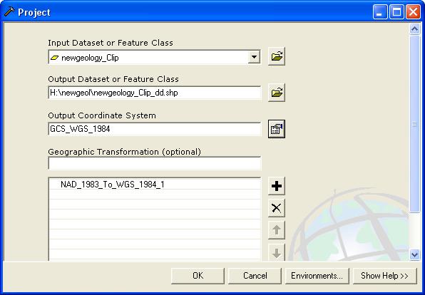
5. Use the Toolbox to project this clipped data to DD.
ArcToolbox->Data Management Tools->Projections and Transformations->Project
Will get you to a screen similar to the following, fill in the values like so, using your own data file names (vegetation_clip, instead of new_geology_clip) and use GCS_Nad83 (import from landslides or new_geology):
Insert a new data frame and put the projected data there. Create a layout showing both versions side-by-side, at the same scale (1:3,000,000 works really well). Comment on the difference...
6. If there is any documentation (metadata)
associated with coverages you download, be sure to save it
along with the data
7. (OPTIONAL)
Do the same with the soils data. Note that it is organized
by county!
Fall 2013: the link on Oregon GIS for Soils is broken,
paste the below link into your browser
http://www.nrcs.usda.gov/wps/portal/nrcs/detailfull/or/soils/?cid=nrcs142p2_045933
Part 2.
8. Go to http://nationalmap.gov/ and use the GIS Data download tool to acquire some 1/3" NED in your study area. You will get a whole 1 x 1 degree area.Get some NAIP imagery (another airphoto) data for a smallish area that has landslides (west hills?) Save them to your C:\temp.
Unzip them.
If you get more than one tile, use the Mosaic To New Raster tool (ArcToolbox->Data Management->Raster->Raster Dataset) to "mosaic them". There is one band in the NED file.Search Help for other mosaic'ing options.
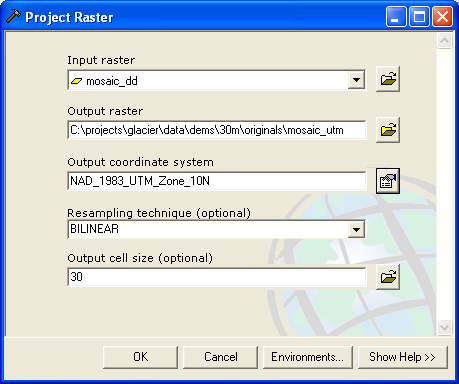
Use ArcToolbox->Data Management Tools->Projections and Transformations->Raster->Project to reproject the NED to UTM zone 10 Nad 83 (must be in planar coordinates to do Surface Analysis), make sure you set your output cellsize to 30m, use Bilinear for the resampling method.
Load Spatial Analyst (Customize->Extensions)
Use ArcToolbox->Spatial Analyst Tools->Surface->Hillshade (accept the defaults) to make a hillshade of your NED. Pay attention to whether your horizontal units match your Z units.
Put your landslides on the hillshade, and the vegetation (try turning on Effects and make vegetation 50% transparent) and admire your pretty map (This is map one: vegetation over hillshade).
Export a PNG of your map to include in your report and then walk away from the data, assuming that the data on the C: drive will be gone when you get back next week.
Next: create a Slope map (Slope tool is near the Hillshade tool) from your UTM-projected data.
Create a contour map (Contour tool found in same place as the others, contour interval depends on zoom-level, try values between 10 and 80) from your DEM.
Create a layout that shows elevation by displaying contours, slope by the default symbolization, and vegetation at 50% transparency. This is a second map for part 2.
Create a map of Topo (DRG) draped over Hillshade, and one
of Airphoto (DOQ) draped over Hillshade. Play with the
transparency settings until it looks pleasing to you.
These are 2 more maps for this section.
For the writeup:
A brief introduction and overview of the assignment
Include the side-by-side layout from step 5 and comments.
Include the FOUR exported maps from step 8 and brief
description of procedure to produce each.