Spatial Statistics of Post-Fire Delayed Tree Mortality to Uncover Ecological Patterns
GEOG 597 Winter 2023 Term Project
Alec Dyer
Monday, March 13, 2023
2020 Labor Day Fires
In September of 2020, several large and severe wildfires occurred in the western Oregon Cascades.
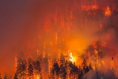
Image courtesy of ESRI & the National Weather Service
Mega-fires
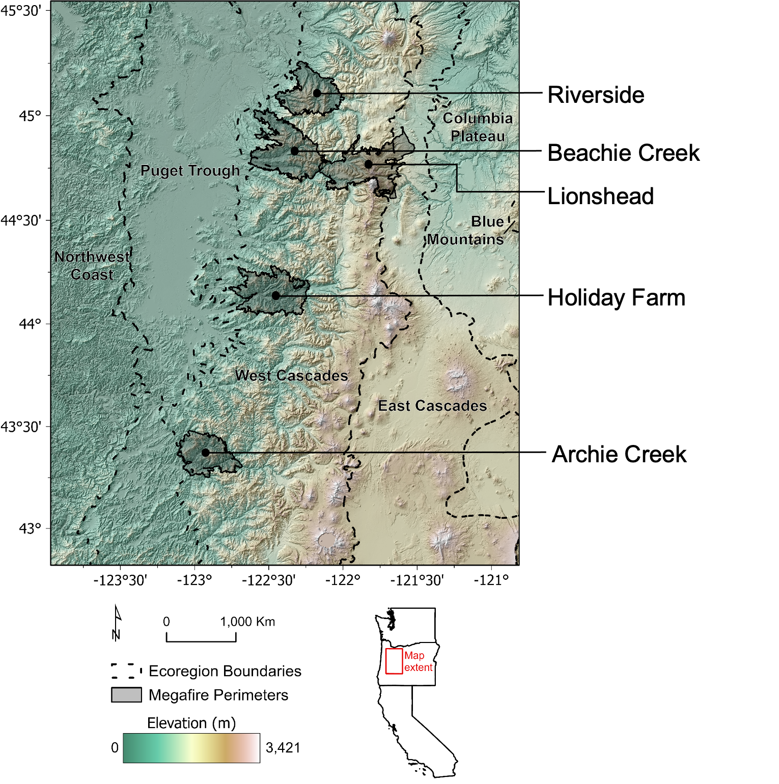
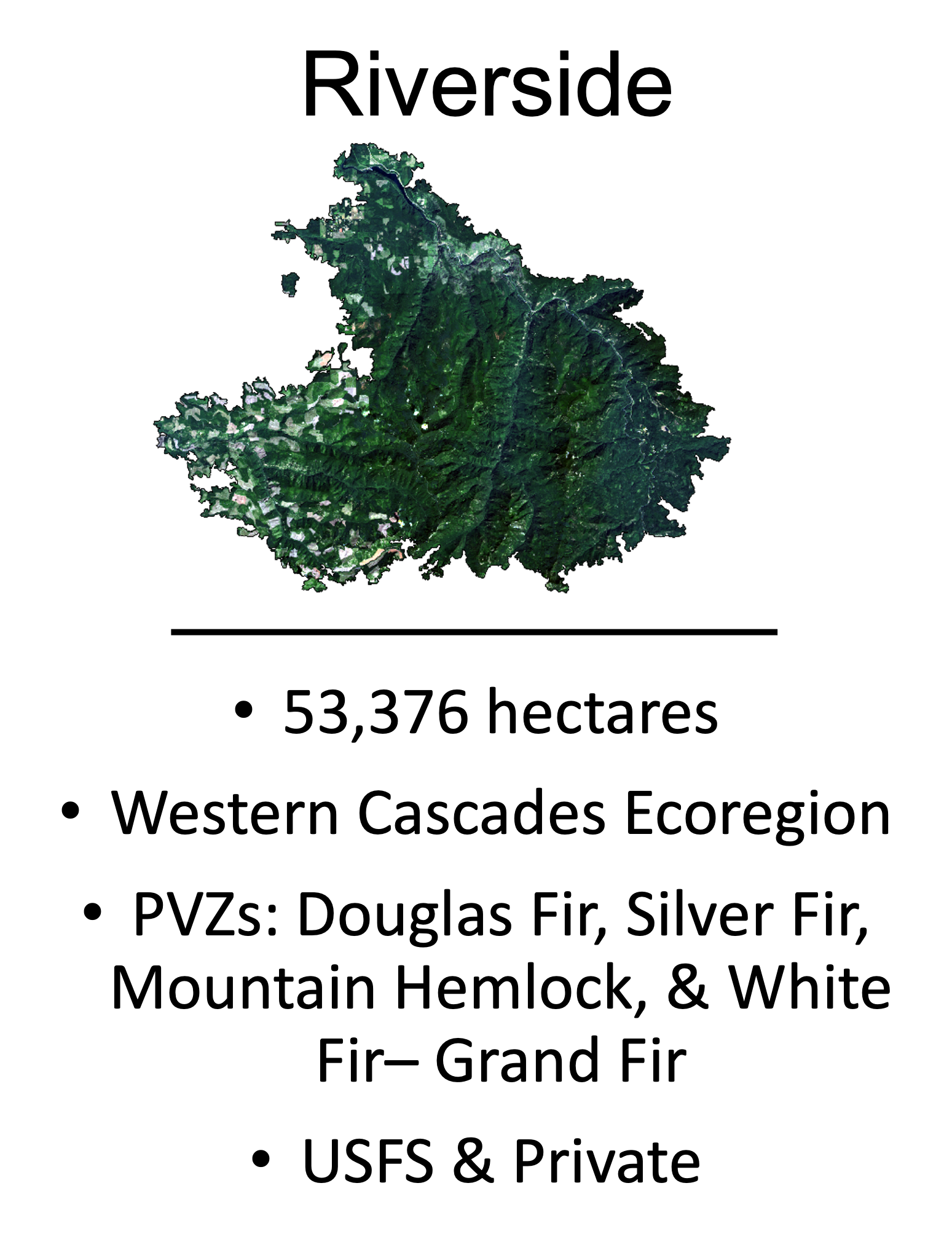
Fire Effects
Immediate Tree Mortality
Using remotely-sensed imagery, immediate post-fire tree mortality can be estimated using formula by Miller & Thode (2007):


Delayed Tree Mortality
The immediate RdNBR formula can be adjusted to estimate delayed mortality:


Research Questions
- Is fire refugia clustered? What are the spatial relationships between severely burned forests and the nearest seed source?
- Is post-fire delayed mortality clustered? What are the spatial & temporal drivers of delayed tree mortality?
Data Setup
Explanatory Variables
Topography
- Elevation
- Slope
- Heat Load Index
Source: Oregon State Service Center for GIS (SSCGIS)
Forest Structure
- Basal Area of Live Trees
- Volume of Live Trees
- Density of Live Trees
- Canopy Coverage
- Mean Stand Age
- Mean Stand Height
Source: LEMMA GNN Forest Structure Data Set
Climate/Weather
Annual measurements betweeen June 1st & August 31st in 2021 and 2022
- Minimum Vapor Pressure Deficit (VPD)
- Maximum Evaporative Demand Drought Index (EDDI)
- Maximum Temperature
Sources: GRIDMET, PRISM
Question #1
Are fire refugia clustered? What are the spatial relationships between highly burned forests and the nearest seed source?
Distance to Seed Source (Refugia)
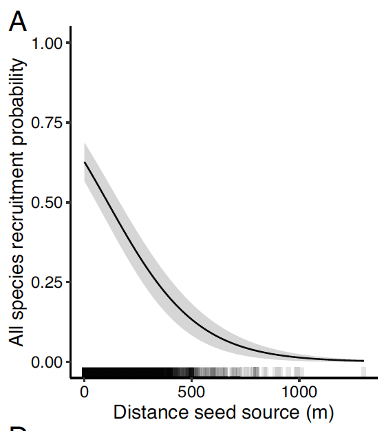
Davis et al., 2023
Refugia Density
# create refugia column where low burn severity (1/0)
pts <- pts %>% mutate(refugia = ifelse(severity %in% c('Low','Moderate'), 1, 0))

# create weights matrix using nearest neighbors within 1000 meters
# dnn <- spdep::dnearneigh(x=pts, d1=1, d2=1000)
# W <- nb2listwdist(neighbours = dnn, pts, type="idw", style="W")
dnn <- readRDS('dnn_matrix.RDS') # load pre-created dnn matrix!
W <- readRDS('dnn_weights_idw.RDS') # load pre-created weights matrix!

pts$refugia_density <- lapply(1:nrow(pts), function(i) {
    r <- pts$refugia[dnn[[i]]]  # get values of nearest neighbor refugia
    w <- W$weights[[i]] # get nearest neighbor weights

    rw <- sum(r*w) # distance-weighted refugia
  }) %>% unlist()

tmap_mode('view')
## tmap mode set to interactive viewingCumulative Refugia Density
ggplot(pts, aes(x=refugia_density)) + stat_ecdf() + theme_bw() + xlab('Refugia Density') + ylab('Cumulative Density (%)')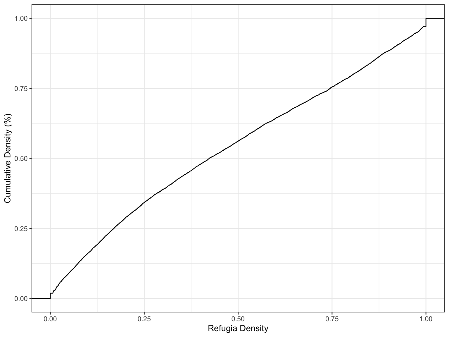
1.9% of the area in USFS land has minimal to zero seed availability for conifer recovery. That leaves a majority of the burned areas suitable for forest recovery.
Is refugia density clustered?
# run global moran's i test for delayed RdNBR 2021
(G_2020 <- moran.mc(pts$refugia_density, W, zero.policy=TRUE, nsim=999, na.action=na.omit))
##
## Monte-Carlo simulation of Moran I
##
## data: pts$refugia_density
## weights: W
## number of simulations + 1: 1000
##
## statistic = 0.91529, observed rank = 1000, p-value = 0.001
## alternative hypothesis: greater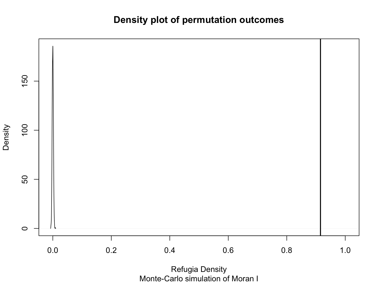
Global Moran’s I results have a p-value of 0.001 and a statistic of 0.915, therefore it can be concluded that refugia density is clustered.
Questions #1 Takeaways
- Fire refugia is spatially clustered, leaving pockets of animal habitat and seeds for neighboring burned patches.
- A majority of the highly burned areas are within 1000 meters of fire refugia.
Question #2
Is post-fire delayed mortality clustered? What are the spatial & temporal drivers of delayed tree mortality?
- Spatial regression
- Random Forest
Spatial Regression
Two response variables:
- Delayed mortality in 2021
- Delayed mortality in 2022
PCA of Delayed Mortality
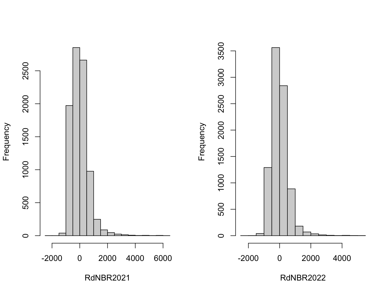
Use PCA to combine delayed RdNBR time periods into a single dimension.
Y <- pts %>% dplyr::select(RdNBR2021, RdNBR2022) %>% st_drop_geometry()
# scale
Y.s <- scale(Y, scale=F)

par(mfrow=c(1,2))
names<-colnames(Y.s)
for (i in 1:ncol(Y.s)) {
  hist(Y.s[,i], main="", xlab=paste(names[i]))
}
Run PCA!
## Importance of components:
##                             Comp.1       Comp.2
## Standard deviation     828.3758703 53.587414125
## Proportion of Variance   0.9958327  0.004167322
## Cumulative Proportion    0.9958327  1.000000000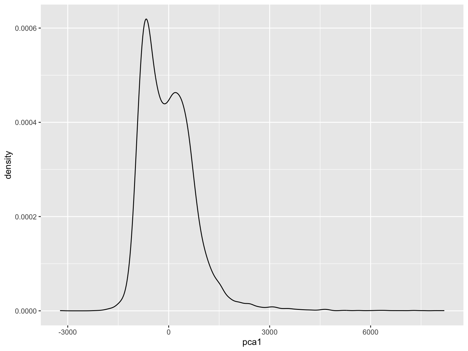
Interpret PC1 using its eigenvectors
## RdNBR2022 RdNBR2021
##      0.66      0.76
Explore the data
Multicollinearity
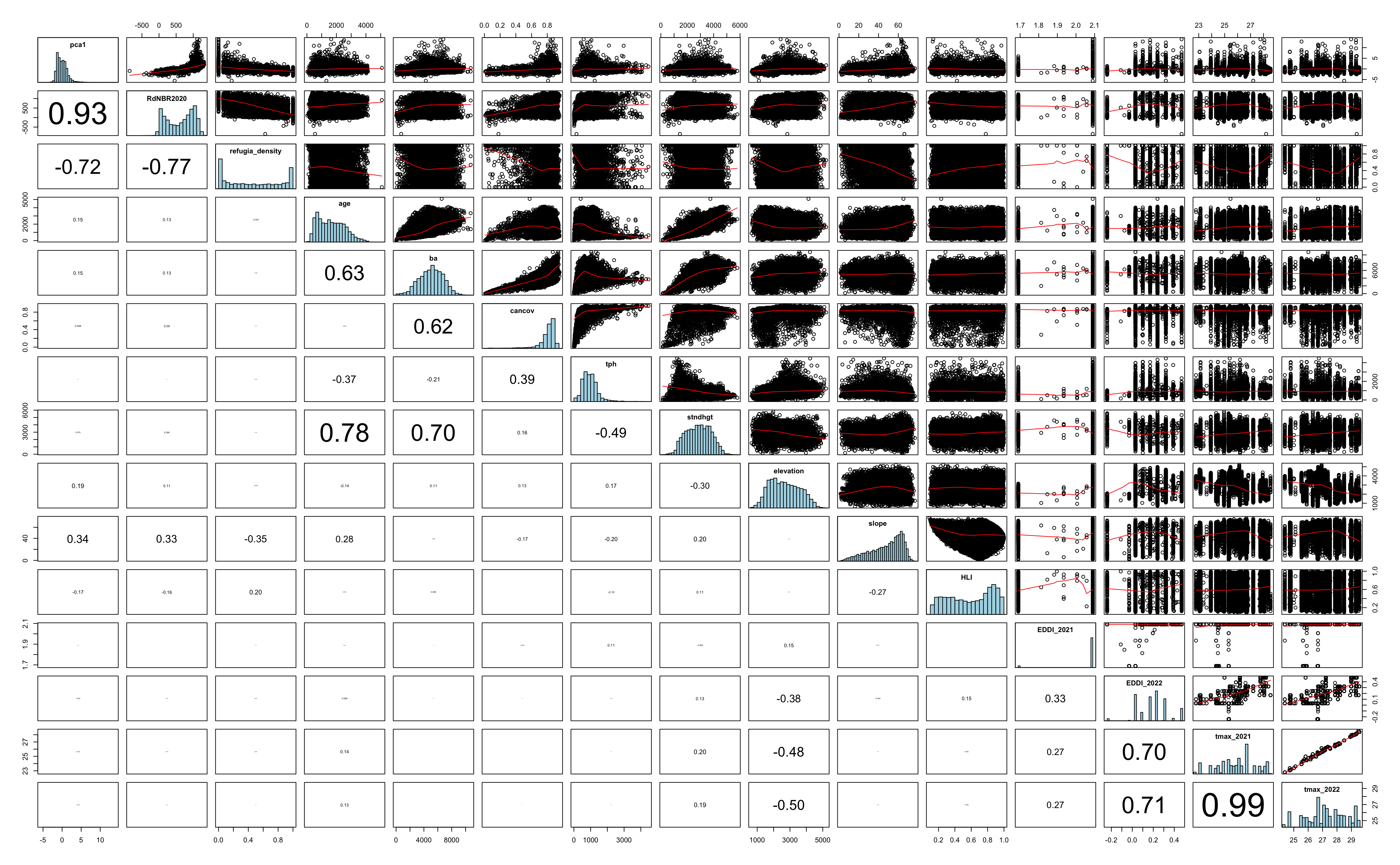
Remove refugia_density, tmax 2022 & stand height
Create OLS model
Delayed RdNBR PCA1 ~ explanatory variables (continous & categorical)
ols_model_pca <- lm(pca1 ~
                  RdNBR2020 +
                  age +
                  basal_area +
                  canopy_coverage +
                  tree_density +
                  elevation +
                  slope +
                  heat_load +
                  EDDI_2021 +
                  EDDI_2022 +
                  tmax_2021 +
                  PVZ +
                  cover_class,

                data = pts)

summary(ols_model_pca, Nagelkerke=T)
##
## Call:
## lm(formula = pca1 ~ RdNBR2020 + age + basal_area + canopy_coverage +
## tree_density + elevation + slope + heat_load + EDDI_2021 +
## EDDI_2022 + tmax_2021 + PVZ + cover_class, data = pts)
##
## Residuals:
## Min 1Q Median 3Q Max
## -2754.5 -219.4 -55.6 126.1 7337.3
##
## Coefficients:
## Estimate Std. Error t value
## (Intercept) -1425.355110 247.452320 -5.760
## RdNBR2020 1.641289 0.014683 111.778
## age 0.007096 0.009270 0.765
## basal_area 0.016372 0.006974 2.347
## canopy_coverage -87.579059 111.638864 -0.784
## tree_density 0.020293 0.015980 1.270
## elevation 0.141536 0.008865 15.965
## slope 0.080803 0.389995 0.207
## heat_load -77.277842 20.919399 -3.694
## EDDI_2021 -41.613436 64.241972 -0.648
## EDDI_2022 -7.284034 51.292892 -0.142
## tmax_2021 16.158498 5.555104 2.909
## PVZMountain Hemlock -418.987435 169.834458 -2.467
## PVZSilver Fir -379.531289 165.729800 -2.290
## PVZWestern Hemlock -307.077940 164.697191 -1.865
## PVZWhite Fir - Grand Fir -365.588850 167.313269 -2.185
## cover_classModerate 36.082979 19.794350 1.823
## cover_classOpen -12.506161 49.885503 -0.251
## cover_classSparse/remnant 192.964411 66.711940 2.893
## Pr(>|t|)
## (Intercept) 0.00000000868 ***
## RdNBR2020 < 0.0000000000000002 ***
## age 0.444002
## basal_area 0.018924 *
## canopy_coverage 0.432776
## tree_density 0.204164
## elevation < 0.0000000000000002 ***
## slope 0.835865
## heat_load 0.000222 ***
## EDDI_2021 0.517156
## EDDI_2022 0.887076
## tmax_2021 0.003638 **
## PVZMountain Hemlock 0.013642 *
## PVZSilver Fir 0.022041 *
## PVZWestern Hemlock 0.062284 .
## PVZWhite Fir - Grand Fir 0.028911 *
## cover_classModerate 0.068353 .
## cover_classOpen 0.802054
## cover_classSparse/remnant 0.003831 **
## ---
## Signif. codes: 0 '***' 0.001 '**' 0.01 '*' 0.05 '.' 0.1 ' ' 1
##
## Residual standard error: 492.1 on 8929 degrees of freedom
## Multiple R-squared: 0.6478, Adjusted R-squared: 0.6471
## F-statistic: 912.5 on 18 and 8929 DF, p-value: < 0.00000000000000022Plot residuals
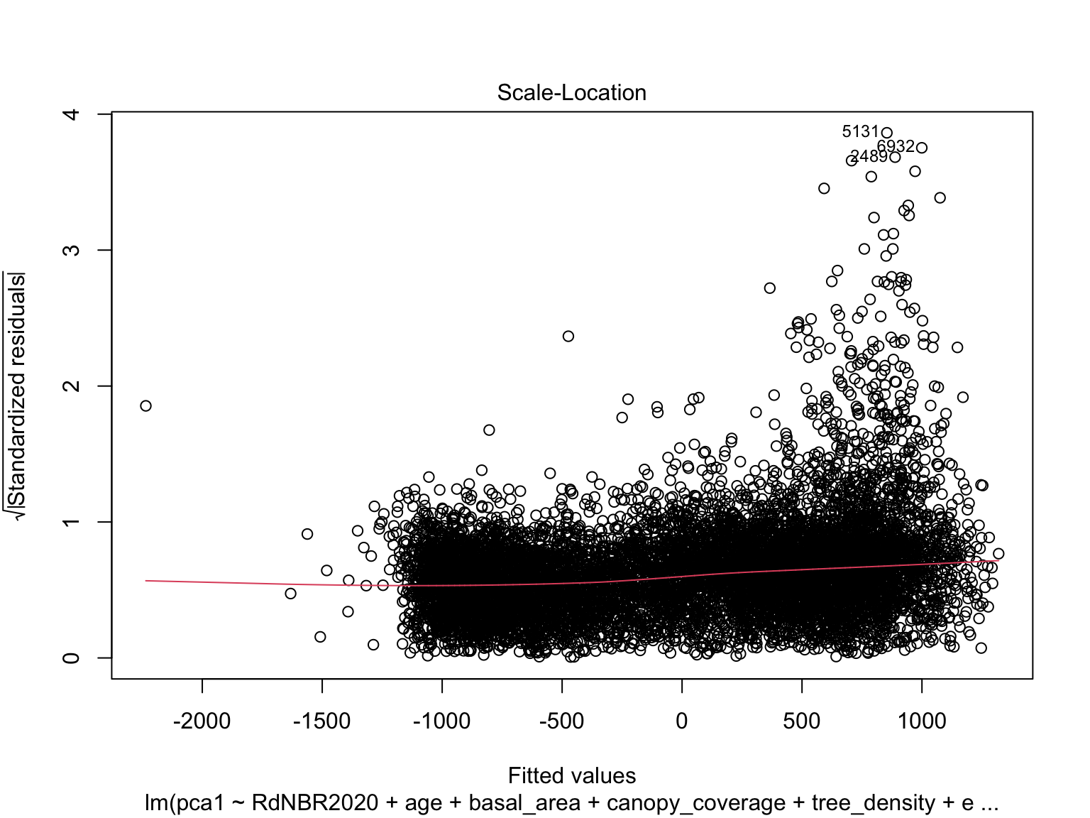
Check Variance Inflation Factor (VIF)
| GVIF | Df | GVIF^(1/(2*Df)) | |
|---|---|---|---|
| RdNBR2020 | 1.223599 | 1 | 1.106164 |
| age | 2.473394 | 1 | 1.572703 |
| basal_area | 5.206075 | 1 | 2.281682 |
| canopy_coverage | 7.290453 | 1 | 2.700084 |
| tree_density | 2.168691 | 1 | 1.472648 |
| elevation | 2.315085 | 1 | 1.521540 |
| slope | 1.495266 | 1 | 1.222811 |
| heat_load | 1.151188 | 1 | 1.072934 |
| EDDI_2021 | 1.248179 | 1 | 1.117220 |
| EDDI_2022 | 2.000404 | 1 | 1.414356 |
| tmax_2021 | 2.317731 | 1 | 1.522410 |
| PVZ | 2.013721 | 4 | 1.091440 |
| cover_class | 3.523028 | 3 | 1.233538 |
Are there spatial autocorrelation in the residuals?
Run Global Moran’s I test
# We have to take into account lm() has dropped entries where any value is NA!
pts$resid_lm_pca[complete.cases(pts %>% st_drop_geometry)] <- ols_model_pca$residuals

# run global moran's i test
moran.mc(pts$resid_lm_pca, listw = W, nsim = 999, na.action = na.omit)
##
## Monte-Carlo simulation of Moran I
##
## data: pts$resid_lm_pca
## weights: W
## number of simulations + 1: 1000
##
## statistic = 0.069527, observed rank = 1000, p-value = 0.001
## alternative hypothesis: greaterSpatial autocorrelation is present in the OLS model residuals.
Lagrange Multiplier
The Lagrange Multiplier (LM) test will be used to determine which spatial model is more appropriate to use.
LM_PCA <- lm.LMtests(model = ols_model_pca, listw = W, test = "all", zero.policy = TRUE)
summary(LM_PCA)
## Lagrange multiplier diagnostics for spatial dependence
## data:
## model: lm(formula = pca1 ~ RdNBR2020 + age + basal_area +
## canopy_coverage + tree_density + elevation + slope + heat_load +
## EDDI_2021 + EDDI_2022 + tmax_2021 + PVZ + cover_class, data = pts)
## weights: W
##
## statistic parameter p.value
## LMerr 1155.11932 1 <0.0000000000000002 ***
## LMlag 137.05798 1 <0.0000000000000002 ***
## RLMerr 1018.61737 1 <0.0000000000000002 ***
## RLMlag 0.55603 1 0.4559
## SARMA 1155.67535 2 <0.0000000000000002 ***
## ---
## Signif. codes: 0 '***' 0.001 '**' 0.01 '*' 0.05 '.' 0.1 ' ' 1The most appropriate spatial model to use is Spatial Error.
Run Regression with Spatial Error Model
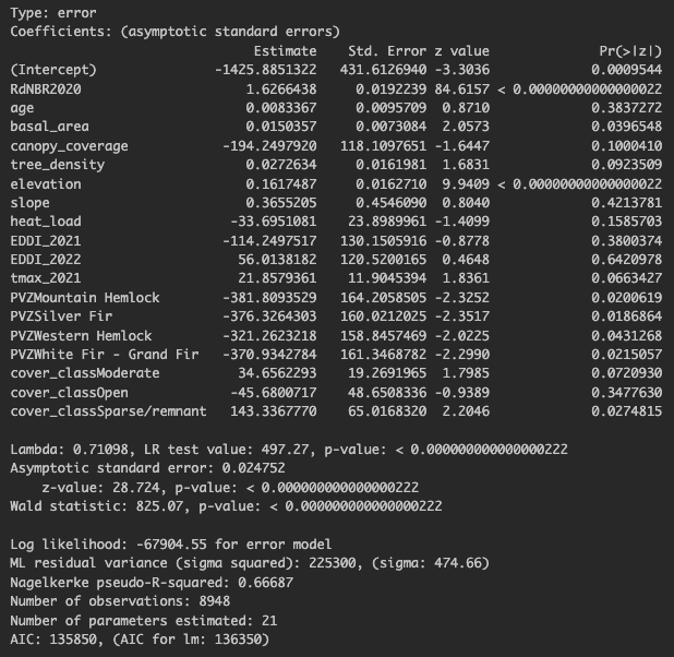
Plot the residuals
mod_err_pca_df <- data.frame('fitted.values'=mod_err_pca$fitted.values,'PCA'=pts$pca1,'residuals'=mod_err_pca$residuals,'standardized.residuals'=sqrt(abs(mod_err_pca$residuals)))

ggplot(mod_err_pca_df, aes(x=fitted.values, y=standardized.residuals)) + geom_point() +
  geom_smooth(method='loess', formula= y~x, color='red')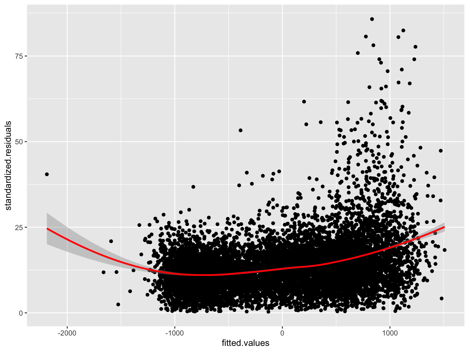
Are the residuals will spatially correlated? Yes… but lower than with the OLS model!
pts$resid_mod_err_pca[complete.cases(pts %>% st_drop_geometry)] <- mod_err_pca$residuals

# run global moran's i test
moran.mc(pts$resid_mod_err_pca, listw = W, nsim = 999, na.action = na.omit)
##
## Monte-Carlo simulation of Moran I
##
## data: pts$resid_mod_err_pca
## weights: W
## number of simulations + 1: 1000
##
## statistic = 0.0047664, observed rank = 986, p-value = 0.014
## alternative hypothesis: greaterRegression Takeaways
- A minimal amount of delayed tree mortality can be explained by the selected topography, forest structure, and climate/weather predictors.
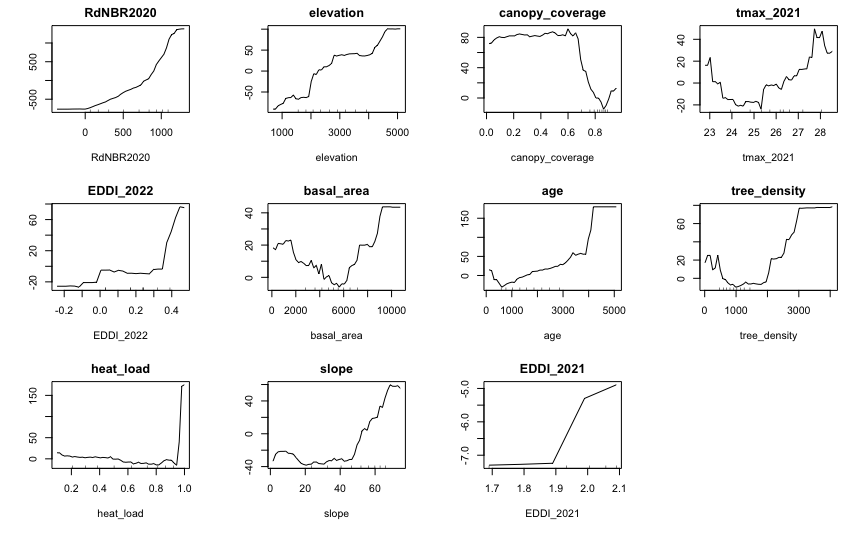
- Immediate tree mortality is a strong predictor of delayed tree mortality.
- Elevation plays a significant role in delayed mortality and can be associated with the characteristics of tree species at different elevation ranges.
Random Forest
Training-Validation Data
set.seed(35)
sub <- sample(
  x = 1:nrow(pts),
  size = floor(nrow(pts) * 0.7),
  replace = FALSE
)

pts_train <- pts[sub,]
pts_test <- pts[-sub,]

paste('Number of Training Observations:', nrow(pts_train))
## [1] "Number of Training Observations: 6263"## [1] "Number of Testing Observations: 2685"Run the Model
Using the same formula for the OLS model, how much more variance in delayed tree mortality can be explained by a RF model?
(pts_rf <- randomForest::randomForest(
  formula = pca1 ~
                  RdNBR2020 +
                  age +
                  basal_area +
                  canopy_coverage +
                  tree_density +
                  elevation +
                  slope +
                  heat_load +
                  EDDI_2021 +
                  EDDI_2022 +
                  tmax_2021 +
                  PVZ +
                  cover_class,
  data = pts_train,
  importance=TRUE,
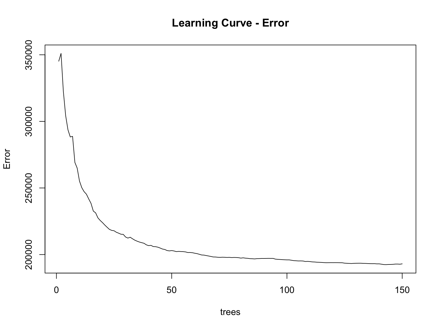
  ntree=150))
##
## Call:
## randomForest(formula = pca1 ~ RdNBR2020 + age + basal_area + canopy_coverage + tree_density + elevation + slope + heat_load + EDDI_2021 + EDDI_2022 + tmax_2021 + PVZ + cover_class, data = pts_train, importance = TRUE, ntree = 150)
## Type of random forest: regression
## Number of trees: 150
## No. of variables tried at each split: 4
##
## Mean of squared residuals: 193033.3
## % Var explained: 71The RF model is able to explain 71% of the variance in delayed tree mortality!
Learning curve
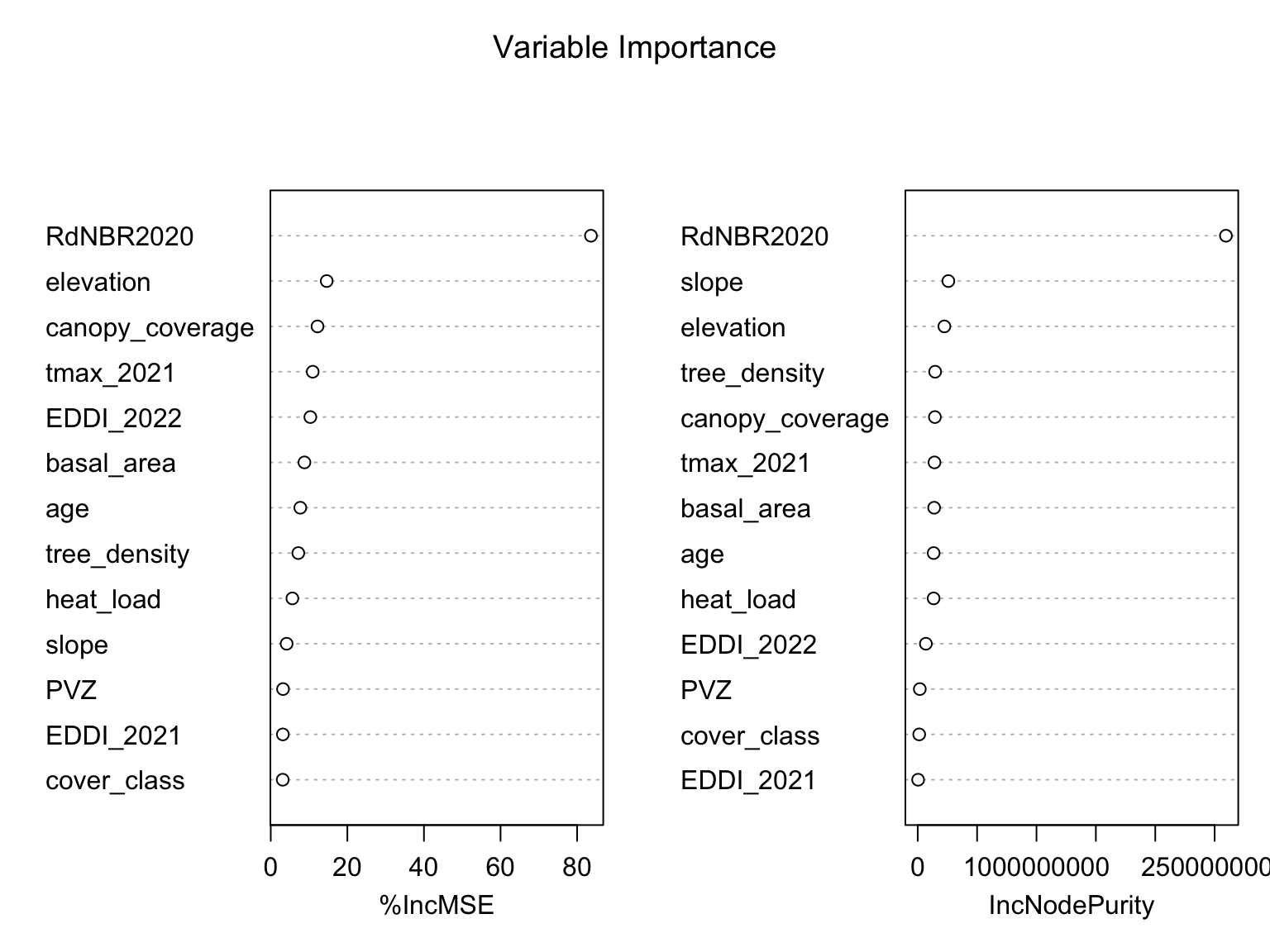
Variable importance
Partial Dependence Plots
Model Evaluation
Evaluate on training and testing data
train_predicted <- predict(pts_rf, pts_train)
pts_train_rf <- lm(pts_train$pca1 ~ train_predicted)

paste('RMSE of training: ', round(sqrt(mean(pts_train_rf$residuals^2)), 2))
## [1] "RMSE of training: 194.47"test_predicted <- predict(pts_rf, pts_test)
pts_test_rf <- lm(pts_test$pca1 ~ test_predicted)
paste('RMSE of testing: ', round(sqrt(mean(pts_test_rf$residuals^2)), 2))## [1] "RMSE of testing: 478.56"Model comparison
How does the RF model compare to the OLS and spatial regression models?
ggplot(model_test_results_df, aes(x=PCA, y=fitted.values, color=model, shape=model)) + geom_point(alpha=0.5) + xlab("Observed") + ylab("Predicted") + geom_abline(intercept = 0, slope = 1, color='black') + theme_bw()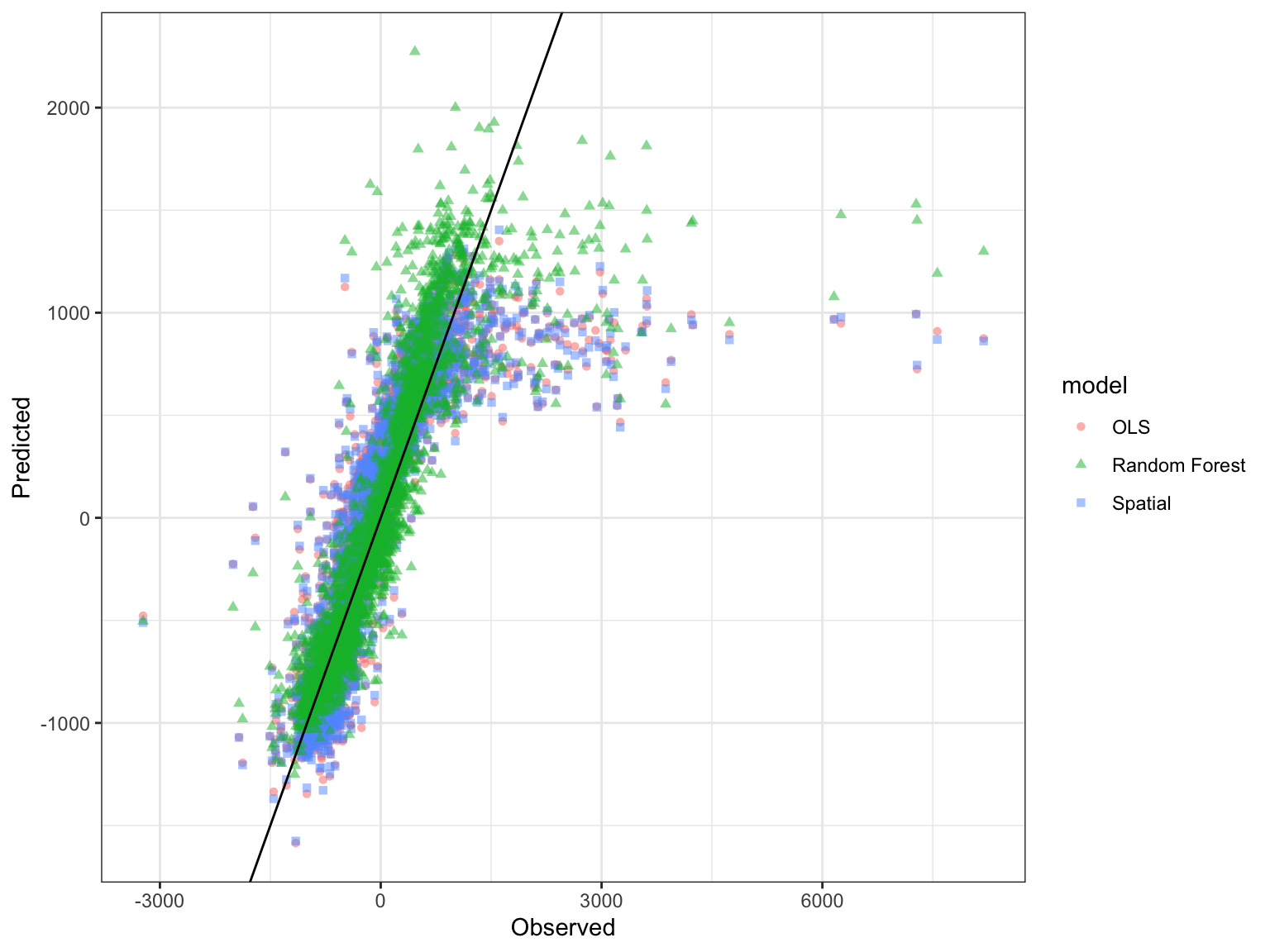
Model comparison of RMSE on the testing set
# RMSE function
calc_rmse <- function(r) { # input residuals
  sqrt(mean(r^2))
}

model_test_results_df %>%
  group_by(model) %>%
  summarize(RMSE = calc_rmse(residuals))
## # A tibble: 3 × 2
## model RMSE
## <chr> <dbl>
## 1 OLS 526.
## 2 Random Forest 479.
## 3 Spatial 527.Model Takeaways
- A Random Forest model can explain more variance in delayed tree mortality compared to OLS and spatial regression models.
- RdNBR outliers are present and significantly affect model performance.
- Immediate burn severity is the strongest predictor of delayed tree mortality in addition to elevation, canopy coverage, & temperature.
Conclusions
- Severely burned patches of forests are within a spatial proximity of fire refugia for successful forest regeneration.
- Spatial patterns are present in delayed tree mortality with increased rates of post-fire decline relating to initial burn severity and physiological characteristics of conifer species.
- The rate of delayed mortality may have increased during the 2021 heat dome event.
- More factors are needed to accurately predict post-fire delayed tree mortality.
References
Abatzoglou, J. T. (2013), Development of gridded surface meteorological data for ecological applications and modelling. Int. J. Climatol., 33: 121–131.
Davis, K. T., Robles, M. D., Kemp, K. B., Higuera, P. E., Chapman, T., Metlen, K. L., et al. (2023). Reduced fire severity offers near-term buffer to climate-driven declines in conifer resilience across the western United States. Proceedings of the National Academy of Sciences, 120(11), e2208120120. https://doi.org/10.1073/pnas.2208120120.
Johnstone, J. F., Allen, C. D., Franklin, J. F., Frelich, L. E., Harvey, B. J., Higuera, P. E., et al. (2016). Changing disturbance regimes, ecological memory, and forest resilience. Frontiers in Ecology and the Environment, 14(7), 369–378. https://doi.org/10.1002/fee.1311.
Landscape Ecology, Modeling, Mapping, & Analysis (2017). GNN Structure (Species-Size) Maps. https://lemma.forestry.oregonstate.edu/data/structure-maps.
Miller, J. D., & Thode, A. E. (2007). Quantifying burn severity in a heterogeneous landscape with a relative version of the delta Normalized Burn Ratio (dNBR). Remote Sensing of Environment, 109(1), 66–80. https://doi.org/10.1016/j.rse.2006.12.006.
PRISM Climate Group, Oregon State University, https://prism.oregonstate.edu, data created 4 Feb 2014, accessed 16 Dec 2020.
Ratajczak, Z., Carpenter, S. R., Ives, A. R., Kucharik, C. J., Ramiadantsoa, T., Stegner, M. A., et al. (2018). Abrupt Change in Ecological Systems: Inference and Diagnosis. Trends in Ecology & Evolution, 33(7), 513–526. https://doi.org/10.1016/j.tree.2018.04.013.
Thank you
Questions?