Lab Exercise 6 - Predator Prey Models

Introduction

Part 1: create the model

The intial equations are:

predator(t) = predator(t - dt) + (predation - pred_loss) * dt
INIT predator = 10

INFLOWS:
predation = harvest_efficiency*predator*prey*(Kpred-predator)/Kpred
OUTFLOWS:
pred_loss = predator*pred_loss_rate
prey(t) = prey(t - dt) + (prey_growth - predation) * dt
INIT prey = 100

INFLOWS:
prey_growth = prey*prey_growth_rate*(200-prey)/200
OUTFLOWS:
predation = harvest_efficiency*predator*prey*(Kpred-predator)/Kpred
harvest_efficiency = .001
Kpred = 200
pred_loss_rate = .1
prey_growth_rate = .1

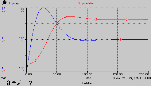
Depending on what you set for the efficiency of the predator-prey interaction (harvest_efficiency) between a value of 0.001 and 0.01, this model will show the following types of behaviors:

damped oscillations to a flat steady state:

 

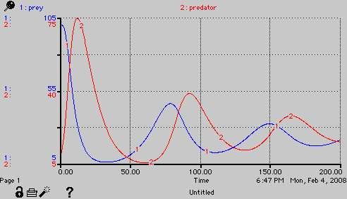
continuing oscillations - but I don't know for how long

 

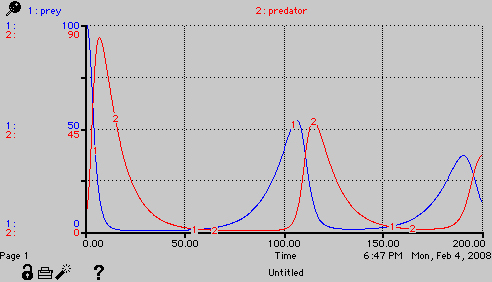
irruption cycles that are clearly separated by recovery periods of low predator and low prey

 

Part one of this assignment is simply to create the model, find values that mimic these different types of curves, and describe what is happening as you change the value of the value of the efficiency.

Part 2: Predator vs. Prey diagrams

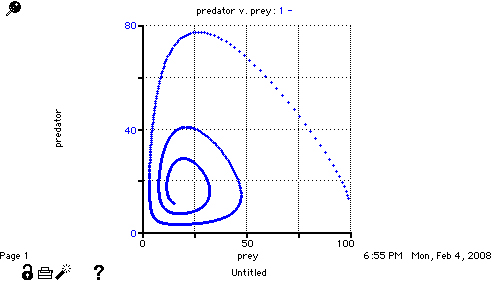
The above diagrams of predator and prey vs. time show show the interaction but you can generate another diagram that illustrates the instantaneous relationship between predator and prey, and by watching this with time you can visualize the impact that each has on the other.

Using the same model as above, create another graph on the page. Double click in this graph and when the dialog box comes up, set the radio button to "scatter graph" and then set the X axis to be prey and the Y axis to be predator.

When you run the model, watch the line develop. You should get a diagram like this for a continuingly damped oscillation.

You might want to slow the simulation down slighlty to visualize where these points are coming from. There are two ways to do this in STELLA. There is a simulation speed slider on the bottom of the model page (I think it has a turtle on one end and a rabbit on the other). The second way is by opening the run-specs dialog box (from the run pull down menu and setting the "sim speed" to something like .1 seconds per time step in the model. In the above case, this would give you a 10 second run to compare the predator and prey vs. time to the predator vs. prey graph.

The assignment is to give one example run from the parameters that cause oscillation and briefly explain what both graphs are showing.