Sampling
This reading is intended to lay out the logic of sampling, and to explain to students who lack statistical training how it is that researchers are able to draw inferences about large populations from relatively small samples.
A problem for your consideration:
A political consultant has two clients, one in Southern California and one in Salem, Oregon. Both candidates are in tight races. Neither candidate wants to fall back on negative campaigning, but if the outcome of the race is uncertain, they would rather resort to a little mud-slinging than risk losing the election. Based on a poll of likely voters, the consultant concludes that each candidate is slightly ahead, 53% to 47%. She bases her estimate of each candidate's strength on the following samples:
L.A. area: 10,000,000 population, sample n = 4,000
Salem area: 100,000 population, sample n = 1,000
Which sample will give the most accurate estimate of the actual level of support for the action? I.e., which candidate can she the most confidently advise that the use of negative campaign tactics should not be necessary?
Answer
Most people will conclude that the Salem sample yields a more accurate estimate and a more confident prediction, because the Salem sample is larger relative to the total population.
Most people will be wrong. The size of the population has nothing to do with it (except for very small populations). The Los Angeles sample will produce twice as accurate an estimate, twice as confident a prediction.
To see why, let's look at some much smaller samples, and a much larger margin of support, for which the math will be easier to understand.
Suppose we find 75% support for a given candidate. We want to know how confident we can be that the observed level of support (the sample statistic) accurately estimates the actual level of support (the population parameter).
We start by testing our observation against an alternative assumption - the null hypothesis.
H1: The true level of support = 75%.
H0: The true level of support is an even split.
Our strategy is to ask, "Suppose the support for our candidate (the population parameter) really isn't any better than 50%. How likely is it that we would observe a sample statistic as high as 75%?"
If opinion is split 50/50, how likely is it that the first person I sample will support my candidate?
How likely is it that each subsequent person will support my candidate?
Notice that each time we draw a new person from the sample, the probability of that person supporting our candidate remains 50%. (Incidentally, that's why I said that this only holds for a relatively large population.)
How likely is it that at least 3 of 4 persons out of the total sample will support our candidate?
Four person sample:
How many possible combinations of opinions can I get?
| First Draw |
Second Draw |
Third Draw |
Fourth Draw |
Sample | Level of Support |
| Y N |
Y N Y N |
Y N Y N Y N Y N |
Y N Y N Y N Y N Y N Y N Y N Y N |
YYYY YYYN YYNY YYNN YNYY YNYN YNNY YNNN NYYY NYYN NYNY NYNN NNYY NNYN NNNY NNNN |
1.00 0.75 0.75 0.50 0.75 0.50 0.50 0.25 0.75 0.50 0.50 0.25 0.50 0.25 0.25 0.00 |
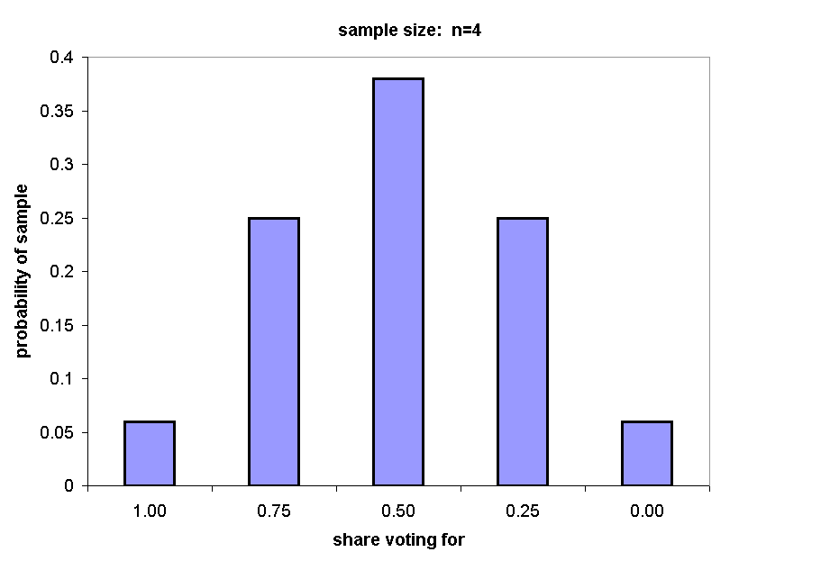
The following chart summarizes the probability of drawing a sample yielding each population statistic, from 0.0% support (p = 1/16, or .0625) to 100% support (p = 1/16, or .0625).

Of 16 equally possible samples, 1 yields 4 supporters and 4 yield 3 supporters. Under H0 (an even split), each sample is equally likely, so the total probability of 75% or more support is 5/16, or .31.
The next chart shows the distribution of possible eight person samples (n = 8).
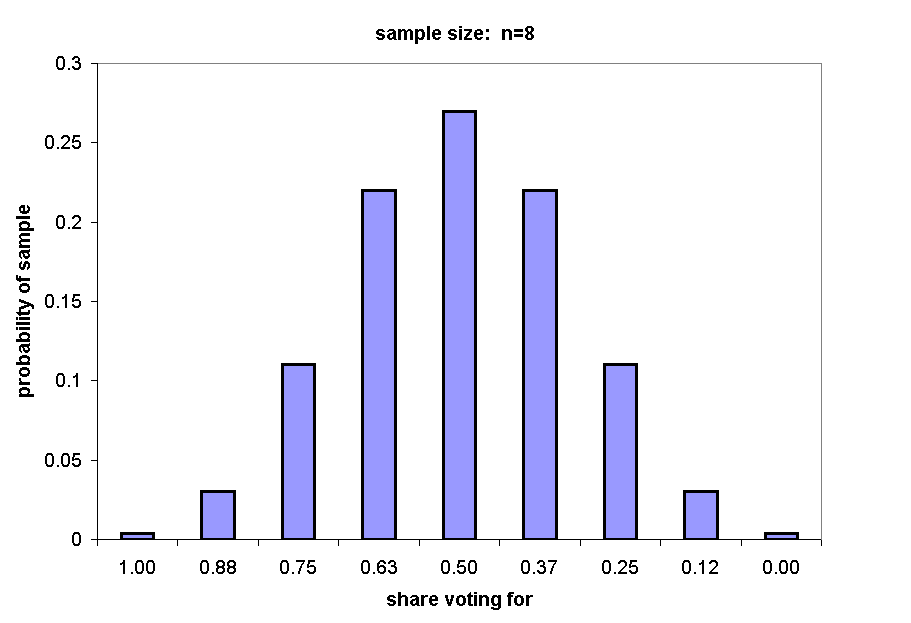
Of 256 total possible samples, 37 (28+8+1) will yield an estimate of 75% or greater: 37/256 = .14.
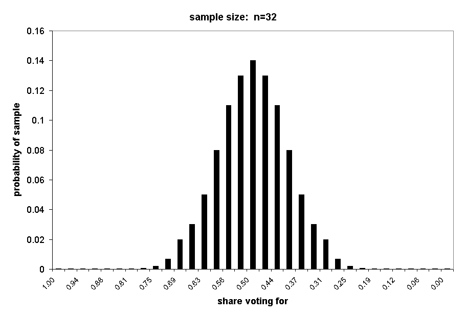
The next three charts show the distributions of samples of n = 16, n = 32, and n = 64.
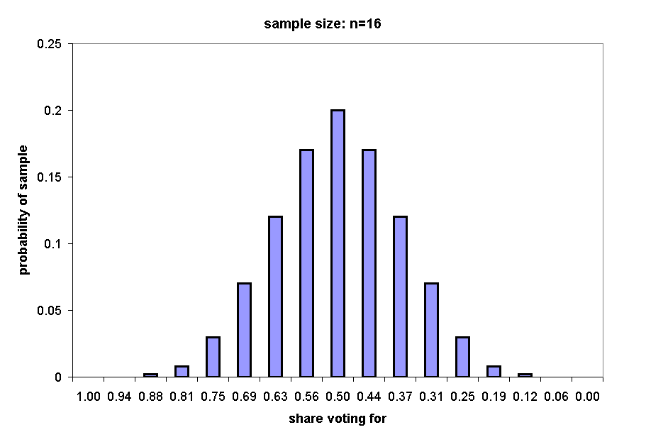
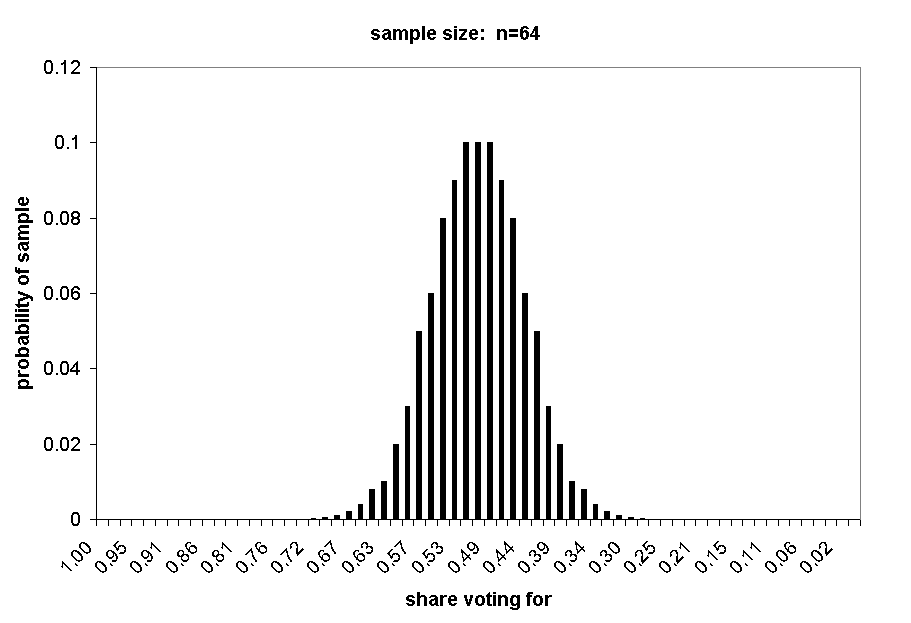
If we draw a sample of 16, there are 216 = 65,536 possible samples, of which a total of 2517 would yield an estimate of 75% or greater: 2517/65536 = .04.
With a sample of 32, the probability of exactly 75% support (24Y) is p = .002. The probability of 75% or more support is a little less than .003.
With a sample of 64, the probability of 75% or more support is less than .0001.
To summarize the precision of different sized samples:
| Sample size | Probability of observed statistic |
| 4 8 16 32 64 |
.31 .14 .04 .0003 .0001 |
Notice what we have computed: We have computed the probability of an actual observation (the sample statistic: 3/4 or more of a sample express support of the war) if an assumption about the population parameter (an even split) is true.
The smaller the probability of the observed sample statistic, the less likely it is that the population parameter is actually as low as 50% - i.e., the more likely it is that more than half the population supports our candidate.
We can turn the logic around, take the sample statistic as an estimate of the population parameter, and calculate a confidence interval within which we expect to find the true population parameter.
To compute a confidence interval, we need two additional concepts, the mean and the standard error.
If we consider all the samples of n = 16 we might draw, the mean is the average of all sample statistics, which we expect to equal the population parameter. For each of our examples, the mean = .75.
The standard error is a measure of how much a typical sample mean will differ from the population mean. For bivariate data (Yes or No), the standard error can be calculated as follows: Where p is the probability of Yes, (1 - p) is the probability of No, and n = the size of the sample,
se = square root of (p*(1 - p) / n)
for n = 4,
se = square root of (.188 / 4)
= sqrt (.188) / sqrt (4) = .44/2
for n = 4, se = .22
for n = 16, se = .11
for n = 32, se = .078
for n = 64, se = .055
As it happens, approximately 95% of all sample means can be expected to fall within two standard errors of the overall mean, 99% of all sample means can be expected to fall within three standard errors of the overall mean. So we can establish a 95% confidence interval (95% CI) as follows: subtract 2se from the mean to find the lower bound, and add 2se to the mean to find the upper bound. To establish a 99%CI, add and subtract 3se to find the lower and upper bounds, respectively.
| sample size | 95% CI | 99% CI | |
| For n = 4 | (.75 + .44) | .32 to 1.0 | .10 to 1.0 |
| For n = 16 | (.75 + .22) | .53 to .97 | .42 to 1.0 |
| For n = 32 | (.75 + .16) | .59 to .91 | .52 to .98 |
| For n= 64 | (.75 + .11) | .64 to .86 | .58 to .92 |
With a sample of n = 16, note that .50 (the null hypothesis) lies outside the 95% CI, consistent with our estimate that the probability of this observation, given the null hypothesis, is less than .05. With a sample of n = 32, .50 also lies outside the 99% CI.
Notice three things:
1. The precision of the estimate increases - and the width of the confidence interval decreases - with the square root of the sample size. To double the precision (halve the width of the CI), you need to quadruple the sample size.
Does the math change if the sample is drawn from a larger population?
2. No. As long as the population is "reasonably large," the precision of the estimate is strictly a function of sample size.
Question: What if I get lazy and draw a sample of convenience:
3. The math depends on the assumption that every member of the population has an equal chance to be sampled! Any deviation from a truly random sample, and the math is meaningless.
Now let's apply this same calculation to our original question. We now know how to establish a 95% or a 99% CI around a sample statistic, based on the observed sample mean and the sample size.
| Study Area (n) | se | Observed | 95% CI | 99% CI |
| L.A. (10mm) . | 008 | .53 | + .016 | + .024 |
| Salem (100k) | .016 | .53 | + .032 | + .048 |
For the Los Angeles candidate, the consultant can report that losing (50% or less of the vote) lies outside the 99% CI - she is 99% confident that the sample mean is an accurate reflection of the true population mean, and that the candidate will win.
For the Salem candidate, the consultant can't even place losing (50% or less) outside the 95% CI. The race is too close to call. The candidate can either dig up the money for a larger sample (if there's still time), or start throwing the mud and deal with the consequences after the election.
The Normal Curve
Our calculations also provide the basis for understanding the famous "normal curve." The next several charts show the distribution of random samples at n = 2 through n = 64. Note how the distribution curves come to approximate a "normal curve" more closely as the sample size increases.