Tutorial on Using NGSpy
Jay Gopalakrishnan
October 2015
Table of Contents
1 What's this?
Relax, NG Spy has nothing to do with Spy ing! We use ngspy or NGSpy to
refer to the python interfaces to Netgen and NGSolve (introduced in
version 6.1).
This is a short introductory tutorial that solves just one problem. The problem is to numerically solve for an electrostatic field using the implementation of the standard finite element method in NGSolve. We begin from the mathematical formulation of the boundary value problem, use the python interfaces to make the required geometry and mesh in Netgen, and then solve the problem in NGSolve.
See this wiki for more tutorials and documentation.
2 The problem
An infinite metallic cylinder, maintained at potential \(u= +1\) Volt, is situated away from a grounded metallic slab at potential \(u=0\) Volt. The potential difference creates an electric field between them. The two-dimensional geometry of the problem is given below.
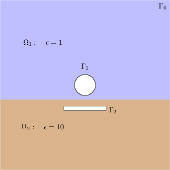
Figure 1: Geometry and notations.
The domain \(\Omega\) (which does not include the circular and rectangular holes) is subdivided into subdomains \(\Omega_1\) and \(\Omega_2\) with different dielectric constants (\(\epsilon\)).
2.1 The equations
The electric field is given by \(E = -\epsilon \nabla u\) where the potential \(u\) solves the following boundary value problem.
\begin{align*} -\mathrm{div}( \epsilon \nabla u) & = 0 && \text{ on } \Omega\\ \frac{\partial u }{\partial n} & = 0 &&\text{ on } \Gamma_0\\ u & =1 && \text{ on } \Gamma_1 \\ u & = 0 && \text{ on } \Gamma_2. \end{align*}2.2 Geometrical dimensions
The dimensions of the geometry we must replicate in Netgen is shown on graph paper below.
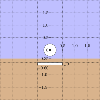
Figure 2: Dimensions in meters
3 Specifying the geometry in Netgen
3.1 Accessing by python
There are several ways to access the Python interface to Netgen and NGSolve:
- Open a terminal and type
netgen. Find the Solve menu item in the top row of the Netgen window, and clickSolve -> Python shell. A python shell will appear in the terminal from which you invokednetgen. The ngsolve python libraries have already been loaded in this python shell. (If your terminal hangs after you quite netgen, typeresetinto the terminal.) - Alternately, you can open a python shell in a terminal and load
netgen and ngsolve. Instead of the simple python shell, you may
prefer to use the enhanced interactive iPython shell (usually
available by typing
ipython3into a terminal). The commandfrom ngsolve import *
will then load all NGsolve objects into your ipython shell.
Your system likely has both Python 2 and Python 3. Beware that in most systems typing
pythonwill only get you Python 2. To use NGSpy you needpython3.
- Another way is to write down all the python commands you want to
execute into a python file, say
script.pyand load it with Netgen by typingnetgen script.pyin the terminal. This is the method we adopt for this tutorial.
3.2 Geometry facilties in NGSpy
We need to tell Netgen about the geometry on which we want to compute.
3.2.1 Lines
- To make the geometry in Figure 2, we need to make the
top and bottom subdomains \(\Omega_1\) and \(\Omega_2\) (which have
different material properties). Let us first make the top
subdomain using
SplineGeometry. Open a python file calledstep1.pyand type these in.from ngsolve import * from netgen.geom2d import SplineGeometry geometry = SplineGeometry()
- Let us first set the geometry to the outer rectangle of
\(\Omega_1\). The outer rectangle has vertices with coordinates
(+2.00,-0.35), (+2.00,+2.00), (-2.00,+2.00) and (-2.00,-0.35),
which we collect into a list
top_pntsby adding these lines.top_pnts = [ (+2.00,-0.35), (+2.00,+2.00), (-2.00,+2.00), (-2.00,-0.35)] top_nums = [geometry.AppendPoint(*p) for p in top_pnts]
Note that the
geometryobject is now aware of these points and has assigned numbers to them, which we can retrieve intop_nums. - Next, we need to make lines connecting these points. A
(directed) line segment is described by one python tuple of the
form
(p0, p1, bn, ml, mr).
The line starts from point p0, ends in point p1, has a number bn used for specifying boundary or interface conditions on this line, and two material numbers ml and mr.
The first material number ml is the number of the material (or subdomain) to the left as we traverse the directed line segment, while mr is material number on the right. Materials outside the computational domain are always marked with material number 0. Hence we set ml to 1 and mr to 0. As for bn, let us set it to some integer, say 10, and proceed. Add these lines to your
step1.py.lines = [ (top_nums[0], top_nums[1], 10, 1, 0), (top_nums[1], top_nums[2], 10, 1, 0), (top_nums[2], top_nums[3], 10, 1, 0), (top_nums[3], top_nums[0], 10, 1, 0) ] for p0,p1,bn,ml,mr in lines: geometry.Append( [ "line", p0, p1 ], bc=bn, leftdomain=ml, rightdomain=mr)
- The
geometryobject now has both the lines and the vertices and is already good for meshing. We callgeometryobject's methodGenerateMesh()and use the output to construct an NGSolveMeshobject, by adding this line tostep1.py.mesh = Mesh( geometry.GenerateMesh() )To check out what we have so far, save
step1.py, open a terminal, and typenetgen step1.py. Clicking on the drop downGeometrybutton in the second menu row of Netgen window will show you the geometry and selectingMeshfrom the drop down menu will display the mesh.
3.2.2 Circular hole
- Although we made and meshed a rectangle above, what we
really wanted to do was to create \(\Omega_1\), a rectangle with
a circular hole. There is no need to throw away your code for
the rectangle. Just put it inside a function like so:
def TopRectangle(geom):

    # Copy over required parts of your code from step1.py.
    # (change geometry to local variable geom)
    # ...
    return geom
- Let us proceed to create the circle using four curved segments. A
(directed) curve is described, just like lines, by one python
tuple of the form
(p0, p1, p2, bn, ml, mr).
The meaning of bn, ml and mr are the same as in the case of line segments. But note that now, instead of two endpoints, a curve is specified by three control points p0, p1, and p2. Namely, the curve begins at p0 and proceeds in the direction of p1, i.e., the tangent to the curve at p0 passes through p1. The curve ends in p2 such that the tangent at p2 also passes through p1, as shown in the figure below.
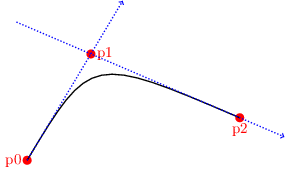
Figure 3: Spline and control points.
Thus, if we set p0=(+0.25, +0.00), p1=(+0.25, +0.25) and p2=(+0.00, +0.25), then we create a circular arc of radius 0.25 in the first quadrant.
- We can now easily make a circular domain of radius 0.25 and
mesh it using the python file circle.py, shown
below:
from ngsolve import *
from netgen.geom2d import SplineGeometry

#--------------------------------------------------------------------
def Circle(geom,r):

    #              point 0   point 1   point 2   point 3  point 4    point 5   point 6   point 7
    disc_pnts = [ ( r,  0), ( r,  r), ( 0,  r), (-r,  r), (-r,  0), (-r, -r), ( 0, -r), ( r, -r) ]

    disc_pnums = [geom.AppendPoint(*p) for p in disc_pnts]

    curves = [ (disc_pnums[0], disc_pnums[1], disc_pnums[2],  1,1,0),
           (disc_pnums[2], disc_pnums[3], disc_pnums[4],  1,1,0),
           (disc_pnums[4], disc_pnums[5], disc_pnums[6],  1,1,0),
           (disc_pnums[6], disc_pnums[7], disc_pnums[0],  1,1,0)  ]

    for p0,p1,p2,bc,left,right in curves:
    geom.Append( ["spline3", p0,p1,p2],
             bc=bc, leftdomain=left, rightdomain=right)
    return geom
#--------------------------------------------------------------------

geometry = SplineGeometry()
geometry = Circle(geometry,0.25)
mesh = Mesh( geometry.GenerateMesh())
Note that we must use
spline3instead ofline. Download circle.py into a folder, go to the folder in a terminal, and typenetgen circle.py. You should see a disc whose inside is meshed. - But we wanted to punch out a disc-shaped hole, not mesh the
disc. No problem: just swap the left and right material
numbers in the list of tuples in
curves. This tells netgen that the inside of the disc is not part of the computational domain (material 0) and that the outside of the disc is material 1. Obviously, we must make sure that there is an enveloping material 1 (otherwise netgen will crash trying to mesh an infinite exterior). - We combine the code for the rectangle and the code of the circle to complete our specification for Ω1 in the file step2.py.
- The final step is to add the subdomain Ω2 and mesh the
composite domain, which I leave as an exercise.
For completing this exercise, it is important to note that you should not add duplicate points or lines in any geometry (i.e., you will have to revise the functions in step2.py). You can find a solution file below, but try it out yourself first.
While you do the exercise, please define a function
MakeMesh()that returns the final mesh (along with other functions it may depend on) inside a file namedmygeom.py. This will be used in the upcoming explanations.
3.3 The old way
There is an alternate way to specify the geometry using a geometry
file in Netgen's 2D geometry input format splinecurves2dv2 (which
works in old and new versions of Netgen). I will not explain this
in detail, but a geometry file is included for completeness. The
comments in this file (on lines beginning with #) are
self-explanatory and will guide you on the usage. To see the
geometry specified by the file, give it to netgen using the menu
option File -> Load Geometry.
4 Solving the boundary value problem
Let us make a new python script for solving the problem, named say
circleplate.py.
- Add this line to the file.
from ngsolve import *
- If you have done the last exercise, then putting the
two statements below into your file will get you the mesh.
from mygeom import MakeMesh

mesh = MakeMesh()
- If you have not done the exercise, then download this prebuilt
mesh file circleplate.vol.gz. Put it in the same folder as your
python file
circleplate.py. Then instead of the statements in Step 2, import the prebuilt mesh bymesh = Mesh("circleplate.vol.gz")
Note that this mesh may look slightly different from the one you built (if you completed your exercise).
4.1 Finite element space
- Finite element spaces are built over meshes. The finite
element space we need for solving the boundary value problem in
Section 2.1 is a Lagrange finite element subspace of the Sobolev space
\(H^1(\Omega)\). If you don't know what this space is, do not worry about it now;
you only need to know that this space contains continuous functions that are
piecewise polynomials on mesh elements. Lagrange finite element spaces are specified in NGSpy as follows.
V = H1(mesh, order=2, dirichlet=[1,2])
Note the options:
order=2specifies that polynomials of degree \(2\) must be used on each mesh element.dirichlet=[1,2]indicates that the only boundary or interface curves that have essential Dirichlet boundary conditions are those which we marked 1 or 2.
- Note that in Section 3.2 we marked the circular hole to 1 and the boundary of the plate to 2. The remainder of \(\partial \Omega\) has the natural Neumann boundary condition. Only the location of essential boundary conditions need to be specified when declaring the finite element space.
4.2 Bilinear form
The finite element approximation to the electrostatic potential, which we continue to call \(u\), satisfies \[ \int_\Omega \epsilon \nabla u \cdot \nabla v \; dx = 0 \] for all \(v\) in V. Note that in our problem, there are no volume sources. The left hand side is a bilinear form of two arguments \(u\) and \(v\).
- To implement this, we first need to specify \(\epsilon\) as
a coefficient function that is constant on each subdomain. In
ngspywe indicate our \(\epsilon\) byepsl = DomainConstantCF([1, 10])
This sets \(\epsilon\) to 1 in the first material and to 10 in the second material.
- Such coefficient functions can be passed to integrators in
NGSolve. One of the many integrators provided is
Laplace. We use it as follows.a = BilinearForm(V, symmetric=True) a+= Laplace(epsl)
The option
symmetricmay be set for efficiency whenever your bilinear form is unchanged when its arguments are swapped.
The object a now can be assembled by a.Assemble(), after
which one can obtain the assembled matrix by a.mat. As always,
in python, you can query methods that a admit by typing
help(a) into an ipython shell (after you make a in the same
shell).
4.3 Extending boundary values
The only sources in our problem are boundary sources. When nonzero Dirichlet boundary conditions need to be imposed, we first extend the boundary data into a grid function \(u_1\) inside the domain. Then the solution \(u\) can be split as \(u = u_0 + u_1\) and we need only solve for \(u_0\) with zero Dirichlet boundary conditions: Namely \(u_0\) in V solves \[ \int_\Omega \epsilon \nabla u_0 \cdot \nabla v \; dx = - \int_\Omega \epsilon \nabla u_1 \cdot \nabla v \; dx \] for all \(v\) in V. Note that the final solution \(u\) is independent of how we perform the extension \(u_1\).
- We need to make an extension \(u_1\). Although our only nonzero boundary condition is \(u=1\) on the circular hole, its simple extension \(u_1 \equiv 1\) everywhere in \(\Omega\) will not do because it does not satisfy the boundary condition \(u=0\) at the plate.
- Another idea that emerges from the facilties we have just seen
is to use this:
extendone = DomainConstantCF([1,0])
The coefficient function
extendoneis indeed an extension of the given boundary values. - However
extendoneis discontinuous and therefore not in V. But NGSpy gives the faciltySetwhich locally projects a given function and averages degrees of freedom to get continuity.u1 = GridFunction(V, name="extension") u1.Set(extendone, BND)
The function
u1is indeed in V. In the python shell typinghelp(GridFunction.Set)will show you that the second argument toSetis abool. By giving the objectBND(imported from NGSolve) we ensure that the projection and averaging occurs only near the boundary. - To visualize the above set
u1, add this line:Draw(u1)
To see the function, save your file
circleplate.pywith the above statements, and typenetgen circleplate.pyinto a terminal. Click theVisualbutton and selectScalar Functiontoextension. You should see a function rapidly cut off to zero from 1 near the circle.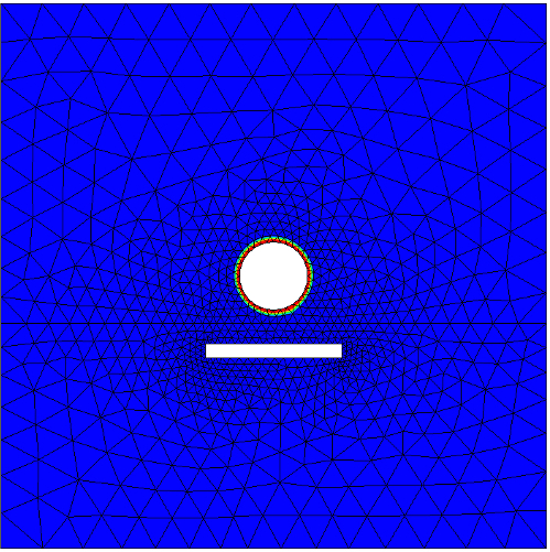
Figure 4: Extension
u1of nonhomogeneous Dirichlet data
4.4 Solving
- We need to invert a linear system and solve for
\(u\). First, allocate space for \(u\).
u = GridFunction(V, name="solution")
u.vec.data = u1.vec
The name of the grid function will be used in visualization menu to identify which function needs to be visualized. The second line copies the contents (the array of values of the coefficients in a basis expansion) of
u1tou. - Next assemble the matrix system.
a.Assemble()
The matrix after assembly is
a.mat. Note that this matrix is built ignoring essential boundary conditions. - The right hand side for the linear system we must
solve is
-a.mat * u1.vec. Space to store this right hand side can be created by asking another vector to clone us a new one.f = u.vec.CreateVector() f.data = a.mat * u1.vec
- Since \(u\) was set to \(u_1\) in Step 12, the final
solution is computed by incrementing the current value of \(u\)
by \(u_0\) after computing \(u_0\) by solving the linear system.
u.vec.data -= a.mat.Inverse(V.FreeDofs(), inverse="sparsecholesky") * f
Draw(u)
The inversion routine uses NGsolve's implementation of a sparse Cholesky factorization algorithm. If you have compiled NGsolve with Intel MKL, then you may have faster options available. The argument
V.FreeDofs()is a bit array that evaluates to true only on unconstrained degrees of freedom. With this argument, the inversion is performed after eliminating the rows and columns of the matrix corresponding to the degrees of freedom constrained by essential boundary conditions.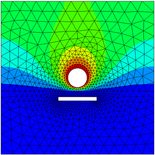
Figure 5: Computed solution
- You can compute and visualize fluxes too.
Draw(-u.Deriv(), mesh, "Flux")The vector field named
Flux, which is the electric field \(E = -\epsilon \nabla u\) in our problem, can now be selected from the Visual menu and visualized either in a quiver plot style or after building field lines. For the quiver plot, chooseVector Functionin theVisualmenu and checkDraw Surface Vectors. For field lines, click onFieldlinesin theVisualmenu.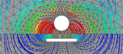
Figure 6: Field lines
- I have collected the above steps to solution into a file circleplate.py which is available for download.
- An alternate way to implement \(u = u_0 + u_1\) is to give
\(u=u_1\) to the built-in facility
BVPwhich then computes and increments by \(u_0\) and outputs \(u= u_0+u_1\). In this method, instead of Steps 14 - 15, we useBVP(bf=a, lf=f, gf=u, pre=c).Do()
If, on input,
ucontains the extensionu1, then on output fromBVPit will contain \(u_0+u_1\). Note that this facility requires you to specify in addition to the bilinear formbf, a linear formlfand a preconditionerc. See the complete file circleplate2.py for details.
5 Files for download
- circle.py: Make a circle
- mygeom.py: Python geometry file for the electrostatics problem
- circleplate.in2d: Geometry file (not pythonic)
- circleplate.vol.gz: Mesh file (not pythonic)
- circleplate.py: Python file to solve the boundary value problem
- circleplate2.py: Alternate python file to solve the same problem
- circleplate.pde: Old PDE style (non-pythonic) input file for solving the same problem.